Component reliability

2. Component reliability#

Task 0: Tasks to complete during the workshop are provided in boxes like this.

In this workshop, we will perform a reliability analysis of a structural problem: the reliability of a short column. In particular, we consider a column subjected to biaxial bending moments \(M_1\) and \(M_2\) and an axial force \(P\) and is illustrated below.

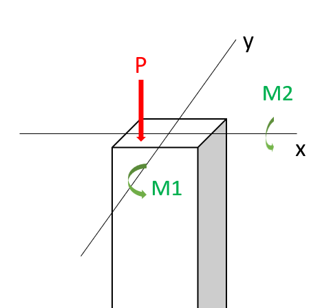
column sujected to biaxial bending

Assuming an elastic perfectly plastic material with yield strength \(y\), the failure of the column is defined by the limit state function:

\[ g(\mathbf{x}) = 1 - \frac{M_1}{s_1 Y} - \frac{M_2}{s_2 Y} - \left(\frac{P}{a Y}\right)^2 \]

where \( \mathbf{x} = \{M_1, M_2, P, Y\}^T \) represents the vector of random variables, \(a=0.190 m^2\) is the cross-sectional area, \(s_1=0.030 m^2\) and \(s_2=0.015 m^2\) are the flexural moduli of the fully plastic column section. Assume \(M_1\) and \(M_2\) are correlated with a coefficient \(\rho=0.5\). The distribution paramaters are given in the table below:

Variable	Marginal distribution	Mean	c.o.v
\(M_1\)	Normal	250	0.3
\(M_2\)	Normal	125	0.3
\(P\)	Gumbel	2500	0.2
\(Y\)	Weibull	40	0.1

We start by importing basic packages.

import numpy as np
import matplotlib.pyplot as plt
import matplotlib.cm as cm

The reliability analysis (FORM) will be performed using OpenTURNS, which is a Python package for reliability analyses. You can read more about the packages or the different functions/classes on their website, or in the tutorial in the Probabilistic Design chapter of the HOS online textbook.

import openturns as ot
import openturns.viewer as viewer
ot.Log.Show(ot.Log.NONE)

The first steps consist in assigning the problem’s variables to python variables:

a = 0.190
s1 = 0.030
s2 = 0.015

You probably observed that the information above contains each distribution’s first and second moments (mean and standard deviation), which for normal distributions is enough to define them on OpenTURNS. However, the Gumbel and Weibull distributions have different distributions parameters, which are defined in OpenTURNS documentation (Gumbel and Weibull). In the context of this workshop, we compute the distribution parameters for you to focus on the analyses; it is however a good exercise to do it yourself later.

The notations adopted below are the one proposed by OpenTURNS and vary from the one of the textbook. Again, mind these differences when using different packages.

The distribution parameters for the Gumbel distribution \(Gumbel(\beta, \gamma)\) are such that:

\[ \mathbb{E}[X] = \gamma + \gamma_e \beta \]

\[ \sigma[X] = \frac{\pi \beta}{\sqrt{6}} \]

# Distribution parameters: P (Gumbel distribution)

beta = (np.sqrt(6)*2500*0.2)/np.pi
gamma = 2500 - np.euler_gamma*beta

Likewise, the distribution parameters for the Weibull distribution \(Weibull(\beta, \alpha)\) are such that:

\( \mathbb{E}[X] = \beta \Gamma \left(1 + \frac{1}{\alpha} \right) \)

\( \sigma [X] = \beta \sqrt{\left(\Gamma \left(1+\frac{2}{\alpha}\right) - \Gamma^2 \left(1 + \frac{1}{\alpha} \right)\right)} \)

By solving the system of equations, we obtain \(\beta = 41700\) and \(\alpha = 12.2\).

We can finally create random variables objects using OpenTURNS and the distribution parameters compute above.

Task 1: Define the marginal distributions of the random variables using OpenTURNS.

M1 = ot.
M2 = ot.
P = ot.
Y = ot.

rho = 0.5    # Correlation coefficient between M1 and M2

  Cell In [6], line 1
    M1 = ot.
            ^
SyntaxError: invalid syntax

As mentioned in the OpenTURNS tutorial, we will be using the PythonFunction class to define our LSF. This requires your LSF to be vectorized, that is allow all the points in a sample to be evaluated without making a for loop : arguments are vectors, returns too.

Task 2: Define the limit-state function.

def myLSF(x):
    ''' 
    Vectorized limit-state function.

    Arguments:
    x: vector. x=[m1, m2, p, y]. 
    '''
    g = [ ]
    return g

Reliability analyses#

Then, we define the OpenTURNS object of interest to perform FORM.

Task 3: Define the correlation matrix for the multivariate probability distribution.

# Definition of the dependence structure: here, multivariate normal with correlation coefficient rho between two RV's.
R = ot.CorrelationMatrix(4)   
R [0,1] = rho
multinorm_copula = ot.NormalCopula(R)

inputDistribution = ot.ComposedDistribution((M1, M2, P, Y), multinorm_copula)
inputDistribution.setDescription(["M1", "M2", "P", "Y"])
inputRandomVector = ot.RandomVector(inputDistribution)

myfunction = ot.PythonFunction(4, 1, myLSF)

# Vector obtained by applying limit state function to X1 and X2
outputvector = ot.CompositeRandomVector(myfunction, inputRandomVector)

# Define failure event: here when the limit state function takes negative values
failureevent = ot.ThresholdEvent(outputvector, ot.Less(), 0)
failureevent.setName('LSF inferior to 0')

---------------------------------------------------------------------------
NameError                                 Traceback (most recent call last)
c:\Users\benja\Documents\TU Delft\Year 2\Teaching Assistant\HOS-prob-design\book\workshops\WS_02_assignment.ipynb Cell 16 in 2
      <a href='vscode-notebook-cell:/c%3A/Users/benja/Documents/TU%20Delft/Year%202/Teaching%20Assistant/HOS-prob-design/book/workshops/WS_02_assignment.ipynb#X21sZmlsZQ%3D%3D?line=0'>1</a> # Definition of the dependence structure: here, multivariate normal with correlation coefficient rho between two RV's.
----> <a href='vscode-notebook-cell:/c%3A/Users/benja/Documents/TU%20Delft/Year%202/Teaching%20Assistant/HOS-prob-design/book/workshops/WS_02_assignment.ipynb#X21sZmlsZQ%3D%3D?line=1'>2</a> R = ot.CorrelationMatrix(4)   
      <a href='vscode-notebook-cell:/c%3A/Users/benja/Documents/TU%20Delft/Year%202/Teaching%20Assistant/HOS-prob-design/book/workshops/WS_02_assignment.ipynb#X21sZmlsZQ%3D%3D?line=2'>3</a> R [0,1] = rho
      <a href='vscode-notebook-cell:/c%3A/Users/benja/Documents/TU%20Delft/Year%202/Teaching%20Assistant/HOS-prob-design/book/workshops/WS_02_assignment.ipynb#X21sZmlsZQ%3D%3D?line=3'>4</a> multinorm_copula = ot.NormalCopula(R)

NameError: name 'ot' is not defined

FORM#

optimAlgo = ot.Cobyla()
optimAlgo.setMaximumEvaluationNumber(1000)
optimAlgo.setMaximumAbsoluteError(1.0e-10)
optimAlgo.setMaximumRelativeError(1.0e-10)
optimAlgo.setMaximumResidualError(1.0e-10)
optimAlgo.setMaximumConstraintError(1.0e-10)

algo = ot.FORM(optimAlgo, failureevent, inputDistribution.getMean())
algo.run()
result = algo.getResult()
x_star = result.getPhysicalSpaceDesignPoint()        # Design point: original space
u_star = result.getStandardSpaceDesignPoint()        # Design point: standard normal space
pf = result.getEventProbability()                    # Failure probability
beta = result.getHasoferReliabilityIndex()           # Reliability index
print('FORM result, pf = {:.4f}'.format(pf))
print('FORM result, beta = {:.3f}\n'.format(beta))
print(u_star)
print(x_star)

Task 4: Interpret the FORM analysis. Be sure to consider: pf, beta, the design point in the x and u space.

MCS#

OpenTURNS also allows users to perform Monte Carlo Simulations. Using the objects defined for FORM, we can compute a sample of \(g(\mathbf{x})\) and count the negative realisations.

montecarlosize = 10000
outputSample = outputvector.getSample(montecarlosize)

number_failures = sum(i < 0 for i in np.array(outputSample))[0]      # Count the failures, i.e the samples for which g(x)<0
pf_mc = number_failures/montecarlosize                               # Calculate the failure probability                       

print("The failure probability computed with FORM (OpenTURNS) is: ",
      "{:.4g}".format(pf))
print("The failure probability computed with MCS (OpenTURNS) is: ",
      "{:.4g}".format(pf_mc))

Task 5: Interpret the MCS and compare it to FORM. What can you learn about the limit-state function?

Importance and Sensitivity#

Importance factors#

As presented in the lecture, the importance factors are useful to rank each variable’s contribution to the realization of the event.

OpenTURNS offers built-in methods to compute the importance factors and display them:

alpha_ot = result.getImportanceFactors()
print(alpha_ot)
result.drawImportanceFactors()

We also compute the importance factors as they are defined in your textbook in order to compare them.

alpha = u_star/beta
print("The importance factors as defined in the textbook are: ", alpha)

The values given by OpenTURNS are completely different than the one calculated above! When using built-in methods, it is essential to check how they are defined, even when the method’s name is explicit.

Bonus: you can figure out the relationship between the textbook’s and OpenTURNS formulation by comparing the package’s documentation and elements of chapter 6 (ADK).

Task 6: Interpret the importance factors. Which random variables act as loads or resistances? What is the order of importance?

Sensitivity factors#

Sensitivity is covered in HW4 and Week 6; it is included here to give you a hint for how it is used in the interpretation of FORM.

We can also access the sensitivity of the reliability index \(\beta\) with regards to the distribution parameters with the built-in method:

sens = result.getHasoferReliabilityIndexSensitivity()
print("The sensitivity factors of the reliability index with regards to the distribution parameters are: ")
print(sens)

Interpretation:

The vectors returned by this method allow us to assess the impact of changes in any distribution parameter on the reliability index, and therefore on the failure probability.

For instance, let us increase the mean of \(M_2\) from 125 to 150. Such change would lead to a decrease of \(\beta\) of \(-0.007 \times 25 = -0.175\). The new failure probability would thus be \( \Phi(-\beta) = \Phi(-(2.565-0.175)) = 0.0084 \), an increase!

Graphical Interpretation#

The difference between the two probabilities above was expected because FORM tends to underestimate the failure probability.

We summarize our findings in two plots. Since \(M_2\) and \(Y\) have the strongest contributions to the failure probability, we choose to position ourselves in that plane first.

Task 7: Complete the code below by filling in the missing values of the design point for the plot. Then take a look at the plots and see if you can learn anything about the limit-state function, and whether it is aligned with your FORM and MCS results. If you were designing a structure using the beam in this proble, would you feel comfortable using the design point from this analysis?

def f_m2(m1, p, y):
    ''' Computes m2 given m1, p and y. '''
    return s2*y - m1*s2/s1 - (s2*p**2) /(y*a**2)

def f_m1(m2, p, y):
    ''' Computes m1 given m2, p and y. '''
    return s1*y - m2*s1/s2 - (s1*p**2) /(y*a**2)



y_sample = np.linspace(10000, 50000, 200)
m1_sample = [f_m1(x_star[1], x_star[2], k) for k in y_sample]     # For now, take (Y, M2) plane

f, ax = plt.subplots(1)

ax.plot(m2_sample, y_sample, label="LSF", color="k")
# Contour plot
X_grid,Y_grid = np.meshgrid(m1_sample,y_sample)
pdf = np.zeros(X_grid.shape)
for i in range(X_grid.shape[0]):
    for j in range(X_grid.shape[1]):
            # This is correct, but only works when ALL RV's are independent!
            # pdf[i,j] = M2.computePDF(X_grid[i,j])*Y.computePDF(Y_grid[i,j])
            pdf[i,j] = inputDistribution.computePDF([X_grid[i,j], x_star[1], x_star[2], Y_grid[i,j]])
ax.contour(X_grid, Y_grid, pdf, levels=8, cmap=cm.Blues)

ax.set_xlabel(r"$M_1$", fontsize=14)
ax.set_ylabel("Y", fontsize=14)

### FILL IN THE DESIGN POINT HERE:
ax.plot( ,  , 'ro', label="Design point")

ylim = ax.get_ylim()
ax.fill_between(m1_sample, ylim[0], y_sample, color="grey", label="Failure region")
ax.set_title(r"Limit state function in the plane $(M_1, Y)$", fontsize=18)
ax.legend();

m1_sample = np.linspace(-300, 500, 200)
m2_sample = [f_m2(k, x_star[2], x_star[3]) for k in m1_sample]

f, ax = plt.subplots(1)

ax.plot(m2_sample, m1_sample, label="LSF", color="k")
# Contour plot
X_grid,Y_grid = np.meshgrid(m2_sample,m1_sample)
pdf = np.zeros(X_grid.shape)
for i in range(X_grid.shape[0]):
    for j in range(X_grid.shape[1]):
            # This is correct, but only works when ALL RV's are independent!
            # pdf[i,j] = M2.computePDF(X_grid[i,j])*Y.computePDF(Y_grid[i,j])
            pdf[i,j] = inputDistribution.computePDF([Y_grid[i,j], X_grid[i,j], x_star[2], x_star[3]])
ax.contour(X_grid, Y_grid, pdf, levels=8, cmap=cm.Blues)

ax.set_xlabel(r"$M_2$", fontsize=14)
ax.set_ylabel(r"$M_1$", fontsize=14)

### FILL IN THE DESIGN POINT HERE:
ax.plot( , , 'ro', label="Design point")

ylim = ax.get_ylim()
ax.fill_between(m2_sample, m1_sample, ylim[1], color="grey", label="Failure region")
ax.set_title(r"Limit state function in the plane $(M_2, M_1)$", fontsize=18)
ax.legend();

Bonus: \(M_1\) and \(M_2\) connected via the Clayton copula#

Note: the dependence structure is quite particular. \(M_1\) and \(M_2\) are correlated, but independent from the other 2 variables (P, Y).

Task 8: You do not need to fill out any code in the bonus part. Take a look at the figures and compare them to the original case, which included linear dependence (i.e., bivariate Gaussian) between the two load variables. Pay particular attention to the correlation structure in both plots, and try to understand where it comes from. Note in particular the commented piece of code, which uses an (incorrect) alternative for computing the PDF. Why is it different, and why is it incorrect? This is especially important for the first plot, which compares two random variables which, based on the correlation matrix, independent.

# Definition of the dependence structure: here, Clayton copula with parameter theta
theta = 2.5
clayton_copula = ot.ClaytonCopula(theta)
indep_copula = ot.IndependentCopula(2)
composed_copula = ot.ComposedCopula([clayton_copula, indep_copula])

inputDistribution_2 = ot.ComposedDistribution((M1, M2, P, Y), composed_copula)
inputDistribution_2.setDescription(["M1", "M2", "P", "Y"])
inputRandomVector_2 = ot.RandomVector(inputDistribution_2)

# Vector obtained by applying limit state function to X1 and X2
outputvector_2 = ot.CompositeRandomVector(myfunction, inputRandomVector_2)

# Define failure event: here when the limit state function takes negative values
failureevent_2 = ot.ThresholdEvent(outputvector_2, ot.Less(), 0)
failureevent_2.setName('LSF inferior to 0')

algo = ot.FORM(optimAlgo, failureevent_2, inputDistribution_2.getMean())
algo.run()
result_2 = algo.getResult()
x_star_2 = result_2.getPhysicalSpaceDesignPoint()
u_star_2 = result_2.getStandardSpaceDesignPoint()
pf_2 = result_2.getEventProbability()
beta_2 = result_2.getHasoferReliabilityIndex()
print('FORM result, pf = {:.4f}'.format(pf_2))
print('FORM result, beta = {:.3f}\n'.format(beta_2))
print(u_star_2)
print(x_star_2)

outputSample = outputvector_2.getSample(montecarlosize)

number_failures = sum(i < 0 for i in np.array(outputSample))[0]      # Count the failures, i.e the samples for which Z<0
pf_mc_2 = number_failures/montecarlosize

print("The failure probability computed using FORM for M1 and M2 having the bivariate normal distribution is: ",
      "{:.4g}".format(pf))
print("The failure probability computed using MCS for M1 and M2 having the bivariate normal distribution is: ",
      "{:.4g}".format(pf_mc))
print("The failure probability computed using FORM for M1 and M2 having the Clayton copula is: ",
      "{:.4g}".format(pf_2))
print("The failure probability computed using MCS for M1 and M2 having the Clayton copula is: ",
      "{:.4g}".format(pf_mc_2))

Let’s redraw our plots from above and see how things are different. Can you tell?

y_sample = np.linspace(10000, 50000, 200)
m2_sample = [f_m2(x_star[0], x_star[2], k) for k in y_sample]     # For now, take (Y, M2) plane

f, ax = plt.subplots(1)

ax.plot(m2_sample, y_sample, label="LSF", color="k")
# Contour plot
X_grid,Y_grid = np.meshgrid(m2_sample,y_sample)
pdf = np.zeros(X_grid.shape)
for i in range(X_grid.shape[0]):
    for j in range(X_grid.shape[1]):
            # This is correct, but only works when ALL RV's are independent!
            # pdf[i,j] = M2.computePDF(X_grid[i,j])*Y.computePDF(Y_grid[i,j])
            pdf[i,j] = inputDistribution_2.computePDF([x_star[0], X_grid[i,j], x_star[2], Y_grid[i,j]])
ax.contour(X_grid, Y_grid, pdf, levels=8, cmap=cm.Blues)

ax.set_xlabel(r"$M_2$", fontsize=14)
ax.set_ylabel("Y", fontsize=14)
ax.plot(x_star[1], x_star[3], 'ro', label="Design point")
ylim = ax.get_ylim()
ax.fill_between(m2_sample, ylim[0], y_sample, color="grey", label="Failure region")
ax.set_title(r"Limit state function in the plane $(M_2, Y)$", fontsize=18)
ax.legend();

m1_sample = np.linspace(-300, 500, 200)
m2_sample = [f_m2(k, x_star[2], x_star[3]) for k in m1_sample]

f, ax = plt.subplots(1)

ax.plot(m2_sample, m1_sample, label="LSF", color="k")
# Contour plot
X_grid,Y_grid = np.meshgrid(m2_sample,m1_sample)
pdf = np.zeros(X_grid.shape)
for i in range(X_grid.shape[0]):
    for j in range(X_grid.shape[1]):
            # This is correct, but only works when ALL RV's are independent!
            # pdf[i,j] = M2.computePDF(X_grid[i,j])*Y.computePDF(Y_grid[i,j])
            pdf[i,j] = inputDistribution_2.computePDF([Y_grid[i,j], X_grid[i,j], x_star[2], x_star[3]])
ax.contour(X_grid, Y_grid, pdf, levels=8, cmap=cm.Blues)

ax.set_xlabel(r"$M_2$", fontsize=14)
ax.set_ylabel(r"$M_1$", fontsize=14)
ax.plot(x_star[1], x_star[0], 'ro', label="Design point")
ylim = ax.get_ylim()
ax.fill_between(m2_sample, m1_sample, ylim[1], color="grey", label="Failure region")
ax.set_title(r"Limit state function in the plane $(M_2, M_1)$", fontsize=18)
ax.legend();