
3.1. Peak Over Threshold (POT)#
The second technique for sampling extremes is Peak Over Threshold (POT). This technique consists of selecting the excesses over a defined threshold with a minimum distance between them. Thus, it involves defining two parameters: the threshold, and the declustering time (minimum time/distance between two extreme observations). Note that when performing EVA with POT, we model the excesses over the threshold, not the actual value of the extreme event.
Let’s apply it to our time series. We are going to use a threshold \(th = 2.5m\) and a declustering time \(dl = 48h\). In the figure below, you can see how the application of this method looks like.
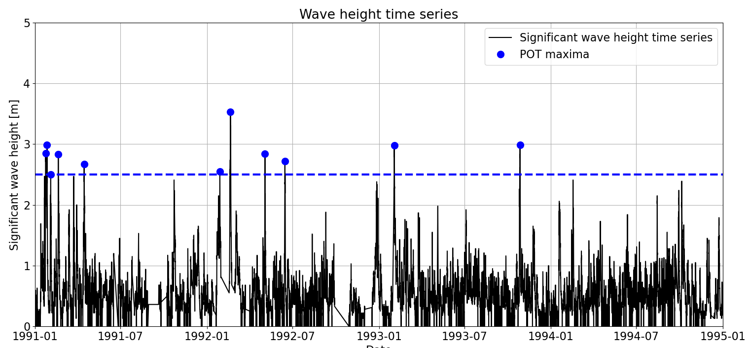
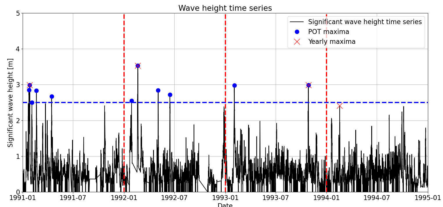
We can see in the figure a concentration of extremes during the first months of 1991 and 1992, even if we have set \(dl = 48h\). When comparing it with Block Maxima (see Figure below), we can see that more extremes are sampled using POT. The main disadvantage of Block Maxima is derived from its simplicity: only one maxima is sampled in each block. Thus, there may be other extreme observations which are not sampled within the same block. Consequently, a higher number of extremes is usually sampled when using POT, although its application is a bit more complicated, as we will see in the following sections. For instance, in our example we obtained 20 extreme observations when applying Yearly Maxima, while we sampled 54 extreme observations when using POT.
Advantages and considerations for use#
We already saw that POT extracts more information from the time series (higher number of extremes sampled), being that a great advantage when working with short time series. However, its implementation is a bit more tricky.
The results of our analysis are dependent on the parameters we select. For instance, if \(th\) is too low, I will be including in the analysis events which cannot be considered extremes. On the other hand, if \(th\) is too high, I will be losing information and, thus, not taking advantage of all the power that POT has. In the following section, we will see tools which support the decision process of determining an appropriate \(th\). However, as a rule of thumb, we can start the analysis using \(th \approx 90-99\) percentile of our observations.
When introducing the concept of \(RT\), we saw that one of the basic assumptions of EVA was that extremes are independent and identically distributed (iid conditions). This implies that when sampling our extremes, we need to ensure that they are independent. At this point is where POT requires a bit more work than Block Maxima: we need to select \(dl\) so we ensure that the sampled observations are independent. Let’s elaborate it a bit more.
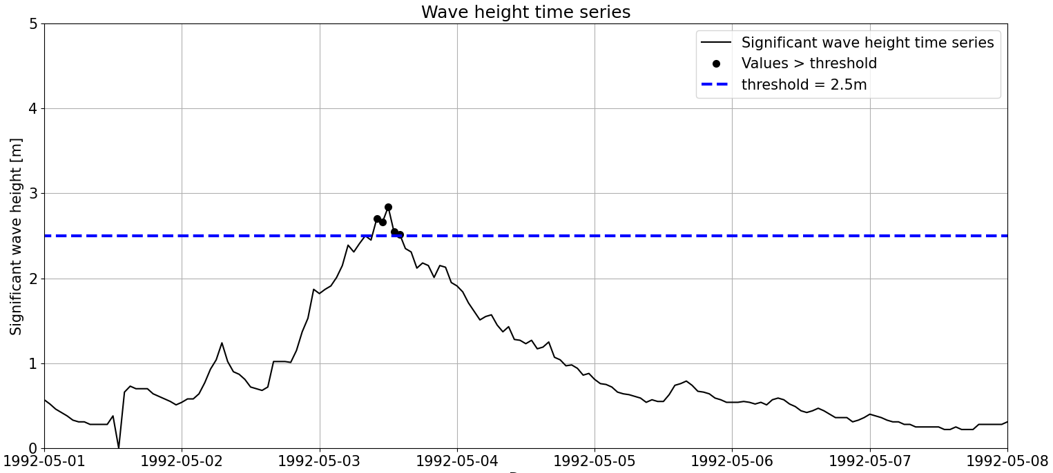
A storm is a phenomenom which lasts several hours, so if we take a look at the time series of hourly \(H_s\) during a storm (see Figure below) we see how registered \(H_s\) goes up, stays around the maximum values for a while and, later, goes down. Therefore, we can say that there is a concentration of extreme values in the storms. For instance, there are 5 observations in a row above \(th = 2.5m\). However, these extremes are caused by the same drivers and are thus dependent. If we included all of them in our EVA analysis, we would be violating the basic assumption of EVA of iid extremes. This phenomenom of concentration of extremes in time is called clustering: we say that extremes cluster in time, since an extreme phenomenom is not composed by a single observation.
And there is where \(dl\) joins the party! If we ensure that the sampled extremes are far enough from each other in time (\(dl\) big enough), we can make sure that they do not belong to the same storm, so we can consider them independent. The needed \(dl\) depends on the physical phenomena which drive the extreme event that we are analyzing and the local conditions. For instance, an appropriate \(dl\) for wave analysis can range from few hours to 72h, since storm duration depends on the local conditions.
In the following sections, we will see how to formally determine the required \(th\) and \(dl\) to ensure that our extremes fulfill the iid assumption.
Peak Over Threshold (POT)
Advantages:
Usually a higher number of sampled extremes. Thus, it is appropriate for shorter time series.
Appropriate when there’s no clear seasonality in the extremes (physical insight in the phenomenom).
Disadvantages:
Further analysis required to ensure that the sampled extremes are iid.
Further computations needed, so the process is slower.
Let’s code it#
In order to exemplify how to actually implement POT,pseudo code is presented.
Pseudo code#
read observations

th = 2.5
dl = 48 #in hours

excesses = find_peaks(observations, threshold = th, distance = dl) - th