
4.3. GPD Parameter Stability#
Another popular graphical method to select the threshold when performing POT is the GPD Parameter Stability plots[1]. This technique is based on the property of GPD distribution of being “threshold stable”. This means that if the exceedances over a high threshold \(th_0\) follow a GPD with parameters \(\xi\) and \(\sigma_{th0}\), then for any other threshold \(th>th_0\), the exceedances will also follow a GPD with the same shape parameter \(\xi\) and a scale parameter \(\sigma_{th}=\sigma_{th0}+\xi(th-th_0)\).
Let \(\sigma^*=\sigma_{th}-\xi th\). Then, \(\sigma^*=\xi th_0\), which does not depend on \(th\) any more.
The parameter stability plot is then defined as
\( \{(th, \sigma^*); th<x_{max}\} \ and \ \{{(th, \xi); th<x_{max}}\} \)
where \(x_{max}\) is the maximum of the observations.
Therefore, \(\sigma^*\) and \(\xi_{th}\) are constant for all \(th>th_0\), if \(th_0\) is a suitable threshold for the asymptotic approximation. This is, the threshold should be chosen so the shape and scale parameters remain constant.
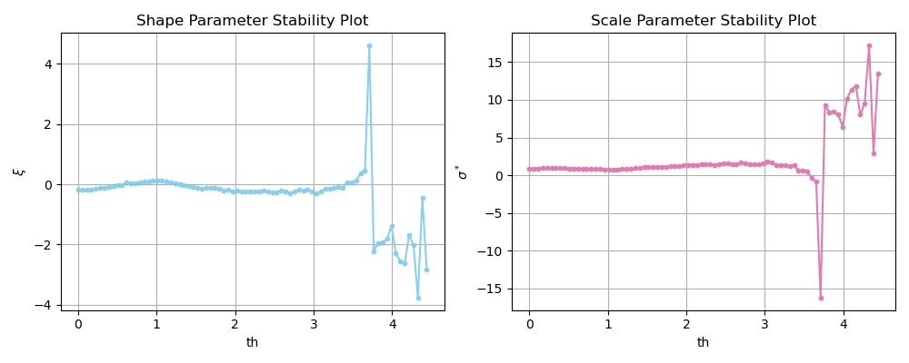
In summary, these plots present in the x-axis different values of \(th\) and in the y-axis the fitted \(\sigma^*\) or \(\xi\) for the values of \(th\) and a value of \(th\) where parameters remain stable should be selected. Note that this is also a graphical method and the interpretation of the analist has a role in the conclusions, being subjected to a certain degree of subjectivity.
In the figure below, you see an application of such method to our \(H_s\) data. We can see that both \(\xi\) and \(\sigma^*\) remain approximately stable for values \(th\leq 3.5m\). Thus, the previously selected \(th=2.5m\) is appropriate considering the Parameter Stability plots.
Let’s code it!#
In order to exemplify how to actually implement GPD Parameter Stability plots, pseudo code is presented. Note that here the first element in a vector corresponds to index 1.
read observations

#define parameters
dl = 48 #in hours
th = linspace(min_threshold, max_threshold, step) #range_thresholds

for i in length(th):
    excesses = find_peaks(observations, threshold = th[i], distance = dl) - th[i]
    scale[i], shape[i] = fit_GPD(excesses)
    modif_scale[i] = scale[1]-shape[i]*(th[i]-th[1])

plot(x = th, y = modif_scale)
plot(x = th, y = shape)