3. OpenTURNS Tutorial

3.1. Introduction

At the moment, this chapter is just a collection of notes from Robert made while using OpenTURNS. The idea is to use it as:

• an introduction to the package OpenTURNS for a new user

• a quick reference for setting up simple analyses

• a help file for students in courses related to probabilistic design at TU Delft

What’s really nice about the package OpenTURNS?

• it has a lot of great analysis tools and a lot of options for modeling probability distributions

• everything is documented well, the code is accessible

• detailed mathematical/theoretical representations, along with a long list of publications

• the classes are robust and make a lot of things very easy!

Disadvantages?

• there’s a bit of a learning curve (hence this document)

• doesn’t follow formatting conventions like PEP-8

Overview of this document

1. Getting started

2. Quick notes: installation, import, sample and point manipulation

3. Example: reliability of a simple slope

4. Example: reliability of a thingamajig

5. Setting up a function and random vectors

6. Reliability analysis of thingamajig with symbolic function (FORM)

Sections 1-4 focus on the structures and methods that make OpenTURNS a powerful probabilistic computational tool, and the examples analyze reliability by directly evaluating the PDF of the limit state function. Sections 5 and 6 illustrate how a Python function or symbolic function can be defined using OpenTURNS, which may be more applicable to problems where the limit-state functions become more complex.

I (Robert) am not a very experience Python user, and my slow progression along the ‘learning curve’ had a lot to do with making errors in generic Python syntax, but also because I skipped reading the explanations of the Point and Sample classes in OpenTURNS, which work in special ways. If you are having trouble making things work in OT, go back and spend some more time on the links and examples in Sections 1 and 2.

3.2. Getting started

It’s easiest to just download ‘exe’ file from github, which installs the package (it worked for me with Anaconda on Windows - choose the right system and Python configuration). See the OT website for other cases.

The default home page is a good place to start exploring, and then is a handy way to find things (along with the quick search). The examples page gives a good overview of key parts of the package. This is important for getting familiar with the special features that OT has, listed below:

• Point and Sample classes: two objects which are essential for using OT and taking advantage of it’s features, but also something that was confusing when I started by jumped straight to examples, so definitely read the explanation first!

• in order to use points and classes like vectors and matrices, they need to be converted to arrays with numpy

• distributions are very easy to specify, and it’s very easy to sample from them

• functions are also very easy to specify, and because it’s so easy to define distributions, it’s also very easy to evaluate them

• many automatic graphing methods

The best way to learn this stuff is to start at the examples page, and don’t skip the topics in data analysis, there are some fundamental lessons there.

Distributions are listed here.

3.3. Quick notes: installation, import, sample and point manipulation

The sample and point classes make it very easy to get samples from a probability distribtuion. The code cells below show how easy it is to define a parametric distribution and draw samples - something that can be done in other Python packages, of course, but these classes are designed to work seemlessly with the more advanced probabilistic methods available in OpenTURNS. This section has the following examples:

• standard packages to import

• quick example of sample and point manipulation, with numpy

• quick example of sample and point manipulation, without numpy

import openturns as ot
import openturns.viewer as viewer
from matplotlib import pylab as plt
ot.Log.Show(ot.Log.NONE)

import numpy as np

x = ot.Normal(4).getSample(6)
print('OpenTurns Sample:\n\n', x)

y = np.array(x)
print('\nOpenTurns Sample converted to numpy array:\n\n', y)

OpenTurns Sample:

     [ X0         X1         X2         X3         ]
0 : [  0.608202  -1.26617   -0.438266   1.20548   ]
1 : [ -2.18139    0.350042  -0.355007   1.43725   ]
2 : [  0.810668   0.793156  -0.470526   0.261018  ]
3 : [ -2.29006   -1.28289   -1.31178   -0.0907838 ]
4 : [  0.995793  -0.139453  -0.560206   0.44549   ]
5 : [  0.322925   0.445785  -1.03808   -0.856712  ]

OpenTurns Sample converted to numpy array:

 [[ 0.60820165 -1.2661731  -0.43826562  1.2054782 ]
 [-2.18138523  0.35004209 -0.35500705  1.43724931]
 [ 0.81066798  0.79315601 -0.4705256   0.26101794]
 [-2.29006198 -1.28288529 -1.31178112 -0.09078383]
 [ 0.99579323 -0.13945282 -0.5602056   0.4454897 ]
 [ 0.32292503  0.4457853  -1.03807659 -0.85671228]]

sample = ot.Normal(4).getSample(6)
print('OpenTurns Sample:\n\n', sample)

OpenTurns Sample:

     [ X0         X1         X2         X3         ]
0 : [  0.473617  -0.125498   0.351418   1.78236   ]
1 : [  0.0702074 -0.781366  -0.721533  -0.241223  ]
2 : [ -1.78796    0.40136    1.36783    1.00434   ]
3 : [  0.741548  -0.0436123  0.539345   0.29995   ]
4 : [  0.407717  -0.485112  -0.382992  -0.752817  ]
5 : [  0.257926   1.96876   -0.671291   1.85579   ]

It’s possible to get one value from a point

print('The second point in the above point is: {0:.3f}'.format(sample[1][1]))

The second point in the above point is: -0.781

Thus it’s also possible to export a point as a list since Samples and Points have list comprehension.

pythonlist = [value for value in sample[1]]
print(f'The second Point has values: ',*[f'{pythonlist:.3f}' for pythonlist in pythonlist])
print('but now it has type ',type(pythonlist))

The second Point has values:  0.070 -0.781 -0.722 -0.241
but now it has type  <class 'list'>

It’s harder to access all points for one of the dimensions from a sample, but fortunately, a Sample has a method asPoint() which gives the values of a 1D sample as a point!

sampleaspoint = sample[:,0].asPoint()
print('\nValues for the first variable are: ',*[f'{i:.3f}' for i in sampleaspoint])
print('with type ',type(sampleaspoint))

Values for the first variable are:  0.474 0.070 -1.788 0.742 0.408 0.258
with type  <class 'openturns.typ.Point'>

3.4. Example: reliability of a simple slope

This is from Baecher and Christian (2003), also used in Moss (2020).

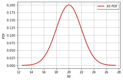
Simple wedge failure with self-weight balanced by cohesion \(c\). Clacluate load as \(S=0.25\gamma H\), where \(h=10\) m. Distributions are normal, where \(\gamma\sim\)N(\(\mu_\gamma=20\) kPa, \(\sigma_\gamma=2\) kPa) and \(c\sim\)N(\(\mu_c=100\) kPa, \(\sigma_c=30\) kPa).

\(Z=R-S=c-0.25\gamma H\)

Results: \(\beta=1.64\) and \(p_f=0.051\).

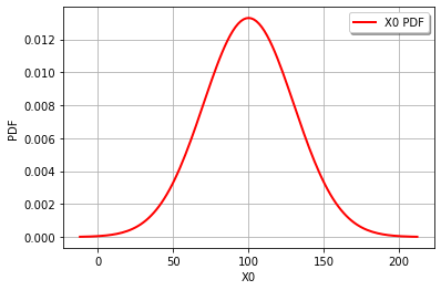
Start by defining the random variables and plotting the distributions.

cohesion = ot.Normal(100,30)
gravity = ot.Normal(20,2)
height = 10

graph = cohesion.drawPDF()
view = viewer.View(graph)
graph = gravity.drawPDF()
view = viewer.View(graph)

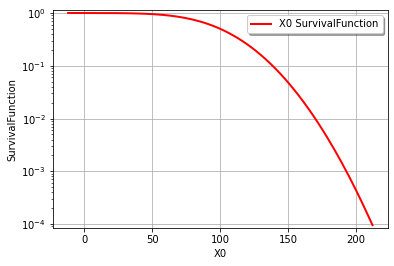
It’s also easy to draw the CDF or inverse CDF and make a logarithmic axis. This page is a good starting point for formatting hints.

graph = cohesion.drawSurvivalFunction()
graph.setLogScale(ot.GraphImplementation.LOGY)
view = viewer.View(graph)

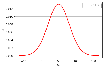
It’s actually very easy to combine distributions in OT. The distribution for a function of random variables (i.e., theoretically and as an OT distribution class) can be evaluated as if they were normal Python variables for addition, multiplication and division using the distributions or scalar values. Thus, for our example, we can combine the distributions for \(R\) and \(S\) directly and solve for the reliability index exactly with just 2 lines. Note: this isn’t just limited to normal distributions, OT can do a lot. See quick start and distribution manipulation example pages. See the transformation page for a list of functions that can be used to transform distributions (e.g., you can’t use \(x^2\), but must use sqr(x)). These functions are methods in the distribution class.

Z = cohesion - 0.25*gravity*height
print('Z becomes a distribution class: ',type(Z),'\n')

beta = Z.getMean()[0]/Z.getStandardDeviation()[0]
pf = Z.computeCDF(0)

print('The reliability index is ',beta)
print('The failure probability is ',pf,'\n')

print('The original distribution for c = ',cohesion)
print('The original distribution for g = ',gravity,'\n')
print('The combined distribution for Z = ',Z)
graph = Z.drawPDF()
view = viewer.View(graph)

Z becomes a distribution class:  <class 'openturns.model_copula.Distribution'> 

The reliability index is  1.643989873053573
The failure probability is  0.050089147113134 

The original distribution for c =  Normal(mu = 100, sigma = 30)
The original distribution for g =  Normal(mu = 20, sigma = 2) 

The combined distribution for Z =  Normal(mu = 50, sigma = 30.4138)

Z = cohesion - 0.25*gravity*height
print(cohesion, gravity, Z)

Normal(mu = 100, sigma = 30) Normal(mu = 20, sigma = 2) Normal(mu = 50, sigma = 30.4138)

3.5. Example: reliability of a thingamajig

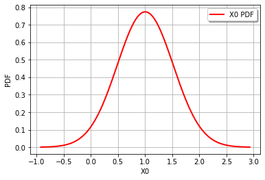
This is from the April 2021 exam for CIE4130 Probababilistic Design, which is looking at the design of a thingamajig. The limit-state function is \(Z=y-x^{0.5}-2\) where \(x\sim\)N\((\mu_x=4.0,\sigma_x=0.5)\) and \(y\sim\)N\((\mu_y=5.0,\sigma_y=0.5)\)

x = ot.Normal(4.0,0.5)
y = ot.Normal(5.0,0.5)
Z = y - x.sqrt() - 2

print('Z becomes a distribution class: ', type(Z), '\n')

beta = Z.getMean()[0]/Z.getStandardDeviation()[0]
pf = Z.computeCDF(0)
pfN = ot.Normal(0,1).computeCDF(-beta)

print('The reliability index is ', beta)
print('The failure probability is ', pf, ', using P[Z<0], whereas')
print('the failure probability is ', pfN, ', using Phi[-beta]\n')

print('The original distribution for x = ', x)
print('The original distribution for y = ', y, '\n')
print('The combined distribution for Z = ', Z)
graph = Z.drawPDF()
view = viewer.View(graph)

Z becomes a distribution class:  <class 'openturns.model_copula.Distribution'> 

The reliability index is  1.947161998215974
The failure probability is  0.025680273921256845 , using P[Z<0], whereas
the failure probability is  0.025757658031434517 , using Phi[-beta]

The original distribution for x =  Normal(mu = 4, sigma = 0.5)
The original distribution for y =  Normal(mu = 5, sigma = 0.5) 

The combined distribution for Z =  RandomMixture(-CompositeDistribution=f(Normal(mu = 4, sigma = 0.5)) with f=[x]->[sqrt(x)] + Normal(mu = 3, sigma = 0.5))

3.6. Setting up a function and random vectors

A random vector is how a random variable is represented. Each variable has an underlying distribution (or several marginals and a defendence structure). A CompositeRandomVector is a function of random variables and is easily defined with the function and RandomVector as inputs. There are several options for specifying a function. See the quick-start guide and other short exmaples described here.

Overview functions

PythonFunction is a class in OT which is defined as follows”

PythonFunction(nbInputs, nbOutputs, myPythonFunc)

where

• nbInputs: the number of inputs,

• nbOutputs: the number of outputs,

• myPythonFunc: a Python function.

Input and outputs are ‘vectors’ (i.e., 1D objects), but inputs are restricted to the OT Point class: y = myPythonFunc(x), thus

def myPythonFunc(x):
    [...]
    return y

Vectorizing the function allows all the points in a sample to be evaluated without making a for loop, but requires conversion to a numpy array. Note: it’s possible to convert all points for each random variable to lists, but I’m not sure if this is more computationally efficient than converting to a numpy array.

import numpy as np

def myPythonFunc(x):
    x = np.array(x)
    x0 = x[:, 0]
    x1 = x[:, 1]
    
    y0 = mysubfunction1(x0, x1)
    y1 = mysubfunction2(x0, x1)
    
    y = np.vstack(y0, y1)
    
    return y

To call a vectorized function, the following func_sample option must be set:

myfunction = PythonFunction(nbInputs, nbOutputs, func_sample = mySimulator)

Symbolic functions can be used to speed up performance and allow derivatives to be computed exactly. The function is defined as follows, with inputs and formulas given as a list of strings:

myfunction = SymbolicFunction(list_of_inputs, list_of_formulas)

Python function and vectorized Python function example

First a Python function. A few notes to remember:

• vectorize input, vector out

• can speed up calculations by allowing the function to take a Sample

• Samples can only handle addition and multiplication, otherwise need numpy (thus only vectorize if calculation is worth the overhead of numpy array conversion; see myLSF2)

• for vectorized functions, use the following option to enable evaluation with a sample, as opposed to a point: func_sample = myfun

Running the two functions below took longer for the vectorized one. Probably because the vector needed to be converted to array and saved.

import time
import numpy as np

# define marginals
x = ot.Normal(4.0, 0.5)
y = ot.Normal(5.0, 0.5)

# multivariate distribution (with independent marginals)
inputDistribution = ot.ComposedDistribution((x, y))
# random vector for generating realizations
inputRandomVector = ot.RandomVector(inputDistribution)

# define the limit-state function
def myLSF(x):
    Z = x[1] - x[0]**0.5 - 2
    y = [Z]
    return y

# create the function of random variables
myfunction = ot.PythonFunction(2, 1, myLSF)
outputvector = ot.CompositeRandomVector(myfunction, inputRandomVector)

# sample
montecarlosize = 10000
t1 = time.time()
outputSample = outputvector.getSample(montecarlosize)
t2 = time.time()

print('Sample mean = ', outputSample.computeMean()[0])
print('Sample stdv = ', outputSample.computeStandardDeviation()[0, 0])
print('calculation took ', t2-t1, ' seconds')

# now create a vectorized function, which requires numpy arrays
def myLSF2(x):
    x = np.array(x)
    Z = x[:, 1] - x[:, 0]**0.5 - 2
    y = np.vstack(Z)
    return y

# create the vectorized Python function using the func_sample option
myfunctionVect = ot.PythonFunction(2, 1, func_sample = myLSF2)
#it is easy to enable the history, but expensive for computation time
#myfunction = ot.MemoizeFunction(myfunction)
outputvector2 = ot.CompositeRandomVector(myfunctionVect, inputRandomVector)

#sample
t1 = time.time()
outputSample2 = outputvector2.getSample(montecarlosize)
t2 = time.time()

print('Sample mean = ', outputSample2.computeMean()[0])
print('Sample stdv = ', outputSample2.computeStandardDeviation()[0, 0])
print('calculation took ', t2 - t1, ' seconds')
# note the way std dev was accessed - as a matrix!

Sample mean =  1.0144595929476583
Sample stdv =  0.524804927305712
calculation took  0.059850454330444336  seconds
Sample mean =  1.0124297386094485
Sample stdv =  0.5211331101231553
calculation took  0.03390836715698242  seconds

It is easy to record and view function inputs and outpus using the function history in the MemoizeFunction class (see Quick-start page). Don’t run it with large samples, though it goes very slow!

Symbolic function example

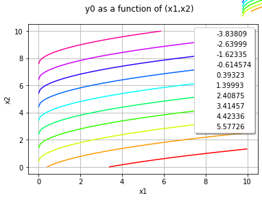
Using the Thingamajig example from above.

Symbolic example page and API page with list of available functions.

# define marginals
x1 = ot.Normal(4.0, 0.5)
x2 = ot.Normal(5.0, 0.5)

# multivariate distribution (with independent marginals)
inputDistribution = ot.ComposedDistribution((x1,x2))
# random vector for generating realizations
inputRandomVector = ot.RandomVector(inputDistribution)

# define the limit-state function
myfunction = ot.SymbolicFunction(['x1','x2'],['x2-x1^0.5-2'])


# create the function of random variables
outputvector = ot.CompositeRandomVector(myfunction,inputRandomVector)

# sample
montecarlosize = 1000
outputSample = outputvector.getSample(montecarlosize)

print('Sample mean = {:.3f}'.format(outputSample.computeMean()[0]))
print('Sample stdv = {:.3f}'.format(outputSample.computeStandardDeviation()[0, 0]))

print('\nThe derivatives are:',myfunction.getGradient())
graph = myfunction.draw(0, 1, 0, [6, 3], [0, 0], [10, 10])
                        #[x1.getMean(),x2.getMean()],
                        #,
                        #)
view = viewer.View(graph)
plt.show()

print([x1.getMean()[0], x2.getMean()[0]])
print(x1.computeQuantile([0.01, 0.99]).asPoint())
print(x2.computeQuantile([0.01, 0.99]).asPoint())

Sample mean = 1.012
Sample stdv = 0.526

The derivatives are: 
| d(y0) / d(x1) = -0.5*x1^-0.5
| d(y0) / d(x2) = 1

[4.0, 5.0]
[2.83683,5.16317]
[3.83683,6.16317]

This is a short example for creating the history, then clearing it and reprinting with only a few samples.

myfunction = ot.SymbolicFunction(['x', 'y'], ['y-x^0.5-2'])
myfunction = ot.MemoizeFunction(myfunction)
outputvector = ot.CompositeRandomVector(myfunction,inputRandomVector)

# sample
montecarlosize=3
outputSample=outputvector.getSample(montecarlosize)

print('Inputs:\n', myfunction.getInputHistory())

outputs = myfunction.getOutputHistory()
print('Outputs:\n', outputs)
print('Number of evaluations of limit state function: ',
      myfunction.getEvaluationCallsNumber(), '\n')

myfunction.clearHistory()

# sample
montecarlosize=5
outputSample = outputvector.getSample(montecarlosize)

outputs = myfunction.getOutputHistory()
print(f'Clear history, then re-run with {montecarlosize} samples:')
print(outputs)
print('Number of evaluations of limit state function: ',
      myfunction.getEvaluationCallsNumber())

Inputs:
 0 : [ 3.67123 4.544   ]
1 : [ 3.81463 5.04689 ]
2 : [ 4.07537 5.11789 ]
Outputs:
 0 : [ 0.627957 ]
1 : [ 1.09378  ]
2 : [ 1.09914  ]
Number of evaluations of limit state function:  3 

Clear history, then re-run with 5 samples:
0 : [ 0.783121 ]
1 : [ 2.01974  ]
2 : [ 1.38774  ]
3 : [ 1.27963  ]
4 : [ 0.6512   ]
Number of evaluations of limit state function:  8

3.7. Reliability analysis of thingamajig with symbolic function

FORM, SORM algorithms here

This page gives a quick-start guide to reliability analysis.

# define marginals
x1=ot.Normal(4.0,0.5)
x2=ot.Normal(5.0,0.5)

# multivariate distribution (with independent marginals)
inputDistribution = ot.ComposedDistribution((x1,x2))
inputDistribution.setDescription(['x1','x2'])

# random vector for generating realizations
inputRandomVector = ot.RandomVector(inputDistribution)

# define the limit-state function
myfunction = ot.SymbolicFunction(['x1','x2'],['x2-x1^0.5-2'])

# create the function of random variables
G = ot.CompositeRandomVector(myfunction,inputRandomVector)
failureevent = ot.ThresholdEvent(G,ot.Less(),0)
failureevent.setName('Thingamajig failure')

optimAlgo = ot.Cobyla()
optimAlgo.setMaximumEvaluationNumber(1000)
optimAlgo.setMaximumAbsoluteError(1.0e-10)
optimAlgo.setMaximumRelativeError(1.0e-10)
optimAlgo.setMaximumResidualError(1.0e-10)
optimAlgo.setMaximumConstraintError(1.0e-10)

algo = ot.FORM(optimAlgo, failureevent, inputDistribution.getMean())
algo.run()
result = algo.getResult()

print('pf = {:.3f}'.format(result.getEventProbability()))
print('beta = {:.3f}'.format(result.getHasoferReliabilityIndex()))
print(result.getStandardSpaceDesignPoint())
print(result.getPhysicalSpaceDesignPoint())

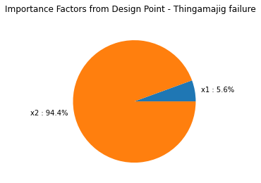
graph = result.drawImportanceFactors()
view = viewer.View(graph)

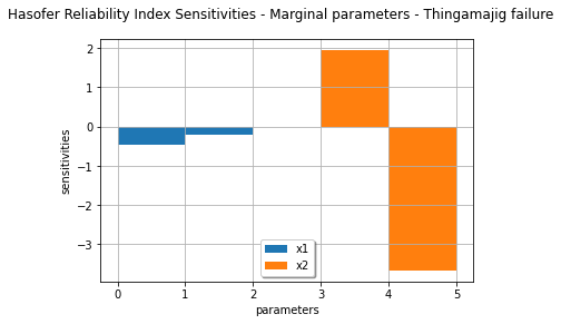
marginalSensitivity, otherSensitivity = result.drawHasoferReliabilityIndexSensitivity()
marginalSensitivity.setLegends(['x1','x2'])
marginalSensitivity.setLegendPosition('bottom')
view = viewer.View(marginalSensitivity)

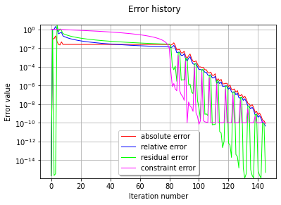
optimResult = result.getOptimizationResult()
graphErrors = optimResult.drawErrorHistory()
graphErrors.setLegendPosition('bottom')
graphErrors.setYMargin(0.0)
view = viewer.View(graphErrors)

pf = 0.026
beta = 1.942
[0.458757,-1.88691]
[4.22938,4.05655]