2.3. GEV Distribution

After sampling the extreme observations in our time series, we want to model the statistical behavior of those maxima. Thus, we are interested in modelling the maximum of the sequence \(X = X_1,...,X_n\), \(M_n = max(X_1,..., X_n)\), where \(n\) is the number of observations in a given block. Assuming that those maxima are independent and identically distributed, we can prove that for large \(n\) the cumulative distribution function of those maxima tend to the Generalized Extreme Value (GEV) family of distributions, regardless the distribution of \(X\).

\( P[M_n\leq x] \rightarrow G(x) \)

Definition and parameters of GEV distribution

Generalized Extreme Value distribution is defined as

\( G(x) = exp{-[1+\xi \frac{x-\mu}{\sigma}]^{-1/\xi}} \hspace{1cm} (1+\xi \frac{x-\mu}{\sigma})>0 \)

where \(-\infty < \mu < \infty\) is the location parameter, \(\sigma > 0\) is the scale parameter, and \(-\infty < \xi < \infty\) is the shape parameter. Let’s see the effect of these parameters the distribution function.

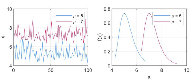
In the figure below, you can see the effect of the location parameter, \(\mu\). A higher value of \(\mu\) leads to a shift towards the right.

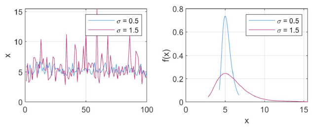
A higher value of the scale parameter, \(\sigma\), leads to a wider distribution, as shown below.

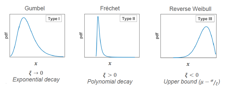
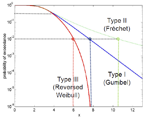
Finally, the shape parameter, \(\xi\), determines the tail of the distribution. This is, the behavior of the distribution at the tail changes based on the value of \(\xi\). If \(\xi \rightarrow 0\), the GEV is called type I or Gumbel distribution and presents an exponential decay at the tail. If \(\xi>0\), the GEV is a type II or Fréchet distribution and the tail presents a polynomial decay. Finally, if \(\xi>0\), the GEV is a type III or Reverse Weibull distribution, and it presents an upper bound.

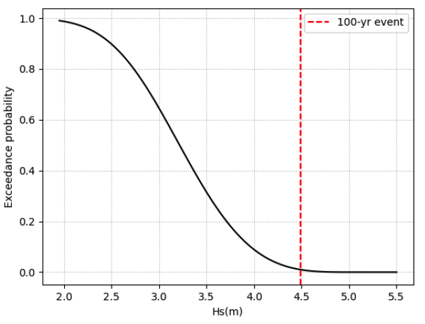
If we plot the exceedance probabilities, we can better see the role of those differences in the tail. Gumbel distribution is said to have a “light tail” since its tail is somewhere in between Reverse Weibull and Frèchet distribution. Small changes in the exceedance probability lead to high differences in the values of the magnitude of interest (\(x\) in the plot below) when analyzing the Frèchet distribution. Indeed, we say it has “a heavy tail”. Finally, for the Reverse Weibull we can clearly see the upper bound around \(x = 8\).

Domains of attraction

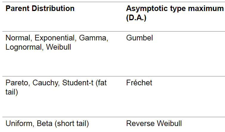
We said that we can prove that for large \(n\) the cumulative distribution function of the values sampled using Block Maxima tend to the Generalized Extreme Value (GEV) family of distributions, regardless the distribution of the \(X\) (parent ditribution). However, we can identify domains of attraction between the parent distributions and the type of GEV or asymptotic type.

Let’s apply it!

Now that you are familiar with the GEV, we can perform the whole EVA process using Block Maxima and GEV and infer extreme values of \(H_s\) that we haven’t observed yet. Remember that in our example we were interested on the value of \(H_s\) for a \(RT = 100\ years\), but we only had 20 years of hourly recordings in our buoy. Thus, we wanted to apply EVA to infer the value of such extreme event for our design. First, we applied Yearly Maxima to sample the extreme observations. Here, we will fit a GEV to those 20 observations and use it to determine the design value of \(H_s\). The process is illustrated using pseudo code below:

read observations 

for each year i:
    obs_max[i] = max(observations in year i) 
end

fit GEV(obs_max)

check fit (e.g., QQ-plot or Kolmogorov-Smirnov test)

inverse GEV to determine the design event

Let’s see it now step by step applied to our data. First, we fit a GEV using MLE to our 20 sampled extremes using Yearly Maxima.

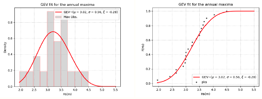
We can see that \(\xi\) is negative, thus it is a GEV type III. Once it is fitted, we need to check how well the theoretical model represents our data. To that end, you can use goodness-of-fit techniques, such as QQ-plot or Kolmogorov-Smirnov test. Here, we assume GEV is a good model and further use it to infer \(H_s\) for a \(RT=100 \ years\).

\(RT = 1/p_{f,y}\), being \(p_{f,y}\) the yearly probability of exceedance. Thus, we need to calculate the value of \(H_s\) with a \(p_{f,y} = 1/100 = 0.01\) or a non-exceedance probability of 0.99. To this end, we can use the inverse of GEV. Working out the equation defining the GEV,

\( z_p = G^{-1}(1-p_{f,y}) = \left\{ \begin{array}{ll} \mu - \frac{\sigma}{\xi}[1-\{-log(1-p_{f,y})\}^{-\xi}] \hspace{1cm} for \ \xi \neq 0\\ \mu - \sigma log\{1-p_{f,y}\} \hspace{2.7cm} for \ \xi = 0 \end{array} \right. \)

Which leads to \(H_{s, RT=100 \ years} \approx 4.5 m\). Congratulations! You have performed your first Extreme Value Analysis!