1. Extremes

If you hear the word “extreme”, the first thing that may come to your mind are extreme sports or natural disasters, such as a hurricane or a typhon. That gives us an intuition of what is an extreme observation in probability theory. Let’s see it in further detail with a dummy example.

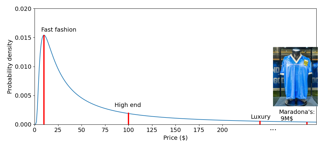
We want to perform a market study of the prices of sold t-shirts to start a new clothing brand. We perform a survey and build the probability density function (pdf) of prices that we can see below. The peak of the distribution, the mode, would correspond to fast fashion brands since they are afordable and sell a lot of product. If we start moving towards the tail, high end brands appear, which are a bit more expensive but still sell a reasonable amount of product. If we keep moving towards the tail, we will find luxury brand which are really exclusive, so they sell little amount of product. Finally, even further in the tail, we would find the world record: the most expensive t-shirt sold in the world, the one which Maradona wore when did the goal with the “hand of God” help, sold by \(\approx\) $9M. It is extreme, right?

Based on the above example, we can define an extreme in probability theory as…

Extreme observation

An extreme is an observation which deviates from the mean and it is thus located at the tail of the distribution.

Why are we interested in extremes?

As engineers, we design interventions and infrastructures to withstand scenarios which are linked to extreme conditions (does it ring the bell “Ultimate Limit State”?). For instance, if we are designing a bridge, we will be interested not only on the daily loads of the cars, but also on the maximum loads that the bridge will face along its design life (e.g.: several large trucks crossing at the same time).

Extreme minimum observations

The critical design condition of a system may be a minimum value. Thus, extremes are not only maxima (e.g.: maximum river discharge or maximum traffic load), but also minima (e.g.: droughts or minimum energy consumption in a network).

As a summary, the first step to properly assess or design a system or infrastructure is to accurately quantify its loads and their uncertainty.

Quantifying extremes using Extreme Value Analysis

Extreme Value Analysis (EVA) allows us to quantify the needed extremes for design. Typically, we have (limited) historical data (e.g.: rainfall data from raingauge stations or wave data from buoys) and we need to quantify extremes which haven’t been observed yet. EVA allows us to model the stochastic behavior of extreme events and infer those which haven’t been observed (extrapolate).

In the following sections, you will see how to select extreme observations within a database (timeseries of observations) and select, fit and use probability distribution functions to characterize their uncertainty and infer the needed extreme values for design.