
4.2. Mean Residual Life#
One of the most popular techniques to select the threshold when performing POT is a graphical method called Mean Residual Life (MRL) plot[1]. MRL plot presents in the x-axis different values of \(th\) and, in the y-axis, the mean excess for that value of the \(th\). The range of appropriate threshold would be that where the mean excesses follows a linear trend.
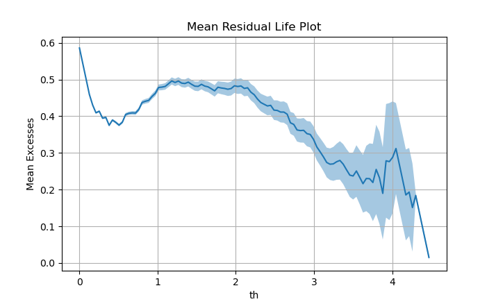
We have computed the MRL plot for our \(Hs\) data and we can see that there is a linear trend from \(H_s \approx 2m\) up to \(H_s \approx 3.5m\). Therefore, our selection of \(th=2.5m\) is appropriate according to the MRL plot. Note that this method is graphical, so it includes a bit of subjectivity.
But what is this based on?#
Let \(Y = [X-th|X>th]\) be the excesses above a threshold \(th\).
Let also \(Y\) be Generalized Pareto (GPD) distributed.
Thus, for every value of \(th^*\geq th\), the excesses \(Y^*= [X-th^*|X>th^*]\) are also GPD distributed with the same shape parameter, \(\xi\), a scale parameter \(\sigma_{th^*}=\sigma_{th}+\xi(th^*-th)\) and a mean value
\( \overline{Y}(th^*) = E[X-th^*|X>th^*] = \frac{\sigma_{th^*}}{1-\xi} \) [2]
Introducing \(\sigma_{th^*}\) into the previous expression, we obtain
\( \overline{Y}(th^*)=\frac{\sigma_{th}+\xi(th^*-th)}{1-\xi}=Ath^*+B \)
being thus \(A=\frac{\xi}{1-\xi}\) and \(B=\frac{\sigma_{th}-\xi th}{1-\xi}\) the slope and intercept of a linear relationship. This means that a linear relationship exists between the mean excesses and the threshold selected when assuming a GPD. Therefore, if we plot the mean excess as function of the threshold, those parts of the plot where a linear relationship is observed are those where it is feasible to apply a GPD.
Let’s code it!#
In order to exemplify how to actually implement MRL plot, pseudo code is presented.
read observations

#define parameters
dl = 48 #in hours
range_thresholds = linspace(min, max, step)

for i in length(range_thresholds):
    excesses = find_peaks(observations, threshold = th[i], distance = dl) - th[i]
    mean_excesses[i] = mean(excesses)

plot(x = range_threshold, y = mean_excesses)