
3.5. GPD: N Return Levels#
Now you know a bit more about the Poisson distribution and how it helps us modelling the number of excesses over a threshold when performing POT. Here, we will see how we can use this distribution to compute the probability of being above the threshold \(P[X>th] = \zeta_{th}\) and, thus, the return levels based on a GPD distribution.
Computing \(N\)-years return levels#
In the previous sections, we reached the following expression to calculate the return levels
\( x_N = \left\{ \begin{array}{ll} th + \frac{\sigma_{th}}{\xi}[(N n_y \zeta_{th})^{\xi}-1] \hspace{1cm} for \ \xi \neq 0\\ th + \sigma_{th} log(N n_y\zeta_{th})\hspace{1.4cm} for \ \xi = 0 \end{array} \right. \)
where \(x_N\) is the \(N\)-years return level, \(th\) the threshold, \(\sigma_{th}\) and \(\xi\) are the fitted parameters of the GPD, \(n_y\) is the average number of exceedances per year and \(\zeta_{th}\) is the probability of observing an exceedance.
We saw that we can model the number of exceedances per year using a Poisson distribution and that this distribution is characterized by a parameter \(\lambda\) equal to the mean and standard deviation of the random variable. Thus, we can calculate \(\zeta_{th}\) [1] as
\( \hat{\zeta}_{th} = \frac{\hat{\lambda}}{n_y} \)
where \(\hat{\lambda}\) can me estimated as the average number of exceedances per year as
\( \hat{\lambda} = \frac{n_{th}}{M} \)
being \(n_{th}\) the total number of sampled exceedances and \(M\) the number of years in the database.
Updating the first equation using the Poisson distribution, we obtain
\( x_N = \left\{ \begin{array}{ll} th + \frac{\sigma_{th}}{\xi}[(\lambda N)^{\xi}-1] \hspace{1cm} for \ \xi \neq 0\\ th + \sigma_{th} log(\lambda N)\hspace{1.4cm} for \ \xi = 0 \end{array} \right. \)
or
\( x_N = \left\{ \begin{array}{ll} th + \frac{\sigma_{th}}{\xi}[(\frac{n_{th}}{M} N)^{\xi}-1] \hspace{1cm} for \ \xi \neq 0\\ th + \sigma_{th} log(\frac{n_{th}}{M} N)\hspace{1.4cm} for \ \xi = 0 \end{array} \right. \)
Let’s apply it!#
Moving back to our example, we were interested in estimating \(H_s\) with a \(RT = 100\ years\). We had 20 years of hourly recordings in our buoy and, using \(th = 2.5m\) and \(dt = 48h\), we sampled 54 excesses.
First, we fit the parameters of our distribution using the sampled excesses, \(\sigma_{th}\) and \(\xi\) using Maximum Loglikelihood Estimator. We obtain \(\sigma_{th}=0.69\) and \(\xi=-0.27\).
Once we have fitted the parameters, we check the goodness of fit of such fitting. Below, the QQplot and the exceedance probability plot in logarithmic scale are presented.
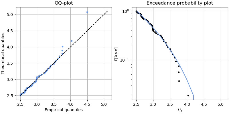
The fitting is reasonable, so we can use the fitted distribution to determine the return level associated to a \(RT = 100 \ years\). We have \(M=20 \ years\) of observations and \(n_{th} = 54 \ events\). Thus, \(\hat{\lambda} = 54/20 = 2.7\). Applying the previous expression for \(\xi \neq 0\)
\( x_{100 \ years} = th + \frac{\sigma_{th}}{\xi}[(\lambda N)^{\xi}-1] = 2.5 + \frac{0.69}{-0.27}[(2.7 \times 100)^{-0.27}-1] = 4.49 \ m \)
Thus, the design wave height with a \(RT=100 \ years\) is 4.49m based on our Extreme Value Analysis. Congratulations! You have performed your first Extreme Value Analysis using POT and GPD!