4.1. Samples: Poisson?

We already applied POT with \(th = 2.5m\) and \(dl=48h\) to our example dataset. Let’s check whether those parameters are appropriate or we should change them. To do so, we are going to check if the number of excesses per year follows a Poisson distribution.

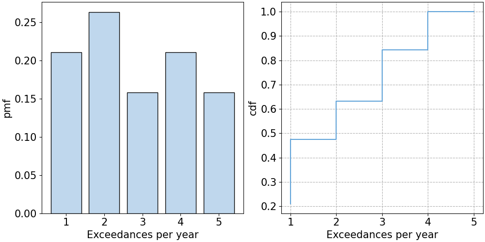
First step is to calculate the number of excesses we have per year and, with it, the empirical pmf and the empirical cdf. Remember that the pmf gives us \(P[X=x]\) and the cdf, \(P[X \leq x]\).

Now, we can fit a Poisson distribution to that empirical distribution and check whether the Poisson distribution is a reasonable model for our number of excesses per year.

We can fit such distribution using L-moments method, which consists of estimating the parameters of the distribution based on the moments calculated from the data (mean, standard deviation…). Applying the properties of the Poisson distribution, \(E[X]=Var[X]=\lambda\), being \(\lambda\) the distribution parameter. Based on that, we can conclude:

• Using my observations, \(E[X]=2.84\) and \(Var[X]= 1.92\). Thus, \(E[X]=Var[X]\) is not true for our observations, but we can assume \(E[X]\approx Var[X]\).

• We can assume a fitted Poisson with \(\lambda = E[X]= 2.84\) for the subsequent analysis.

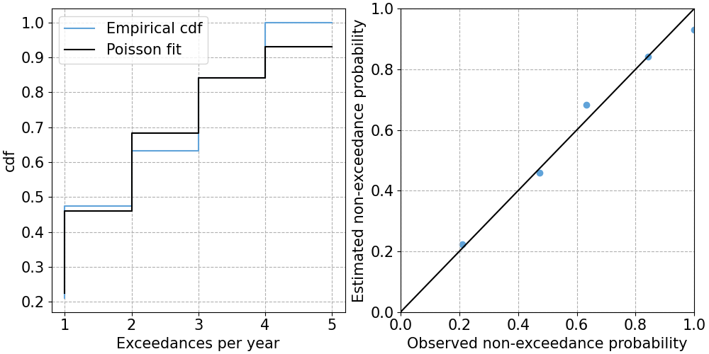
Once we have fitted the Poisson distribution, we can visually check the fit, as shown below. The figure on the left shows the supperposition of the empirical and fitted cdf. The figure on the right shows the empirical and estimated probabilities for number of excesses = 1, 2, … 5, namely the PP-plot. The fitting seems reasonable.

In order to further support our decision, we can perform a goodness-of-fit hypothesis test for discrete distributions, such as \(\chi^2\) test.