
2.2. Asymptotic Model#
In the previous section, we have seen the first technique to sample extreme observations: Block Maxima. But which distribution do these extreme observations follow? In order to better answer this question, here we introduce the asymptotic model.
Asymptotic model
Given \(X = (X_1, X_2, ..., X_n)\) as a sequence of independent and identically distributed random variables which follow the distribution function \(F(x)\).
Being the maximum of the process \(M_n=max(X_1, X_2, ..., X_n)\)
The theoretical distribution of \(M_n\) is \(F(x)^n\)
We can prove it by calculating the probability of the maxima of the sequence (\(M_n\)) being lower or equal than \(x\). If the maximum value of a sequence is below a given \(x\), all the values of the sequence will also be below such \(x\). Thus, it is the same as calculating the probability of each value of the sequence \(X\) being lower of equal than \(x\). Since we have stated that \(X\) is a sequence of independent and identically distributed observations, the joint probability can be computed as the product of the individual probabilities. Hence, the distribution of the extremes is \(F(x)^n\).
\( P[M_n \leq x] = P[max(X) \leq x] \\ = P[X_1 \leq x, ..., X_n \leq x] \\ = P[X_1 \leq x] ... P[X_n \leq x] = F(x)^n \)
Let’s see it with an example!#
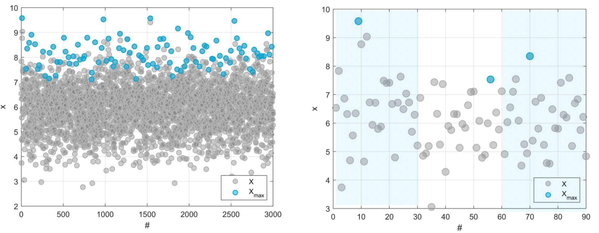
We are going to generate 100 samples with length N = 30 using a Normal distribution \(N(6,1)\). From each sample (block), we are going to store the maximum observation (\(x_{max}\)). Note that we are applying Block Maxima here. In the figure below, you can see in grey the full samples and in blue the maxima from each sample.
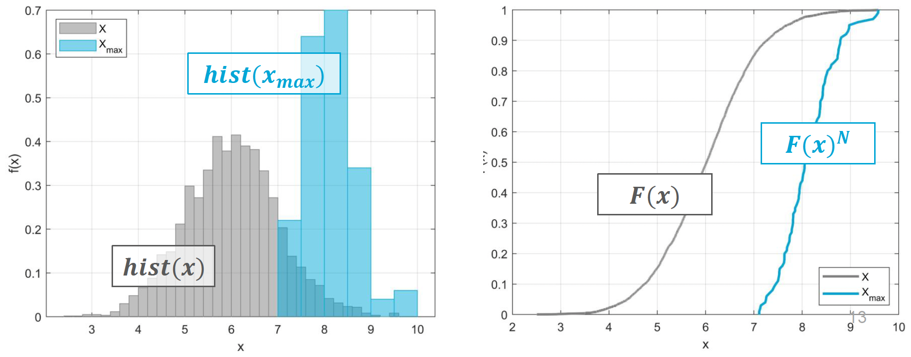
If we plot the histogram of the samples and the plot of the maxima from each sample (see left image below), we can see that the histogram of the maxima is placed on the right tail of the histogram build with all the samples. Also, in the empirical cumulative distribution function (cdf) plot, we can see that the samples follow a \(F(x) \sim N(6, 1)\) as expected, while the maxima follow \(F(x)^n\) as we previously stated.
In pseudo code#
If you want to repeat that analysis yourself, you can do it implementing the following pseudo code.
mu = 6
sd = 1
N = 30
for i in range(100):
    x[:,i] = normal.random(mu, sd, N)
    x_max[i] = max(x[:,i])
end

plot histogram(x), histogram(x_max)
plot ecdf(x), ecdf(x_max)