
4.4. Dispersion Index#
An alternative way of checking that the sampled excesses over a threshold approximate a Poisson process is the Dispersion Index (\(DI\)) [1]. Remember that we wanted the number of excesses per year (or any other time block) to follow a Poisson distribution, \(X \sim Poisson(\lambda)\). The \(DI\) is defined as the intensity or rate of the Poisson process, \(\lambda\) over the mean of the number of excesses per year, \(\mu = E(X)\). By definition in a Poisson process [2], the rate is equal to the variance of the process, \(\lambda = \sigma^2\). Thus, the \(DI\) can be calculated as
\( DI=\sigma^2/\mu \)
where \(\sigma^2\) and \(\mu\) are the variance and mean of \(X\).
Also, by definition, the rate in a Poisson process is equal to the mean, \(\lambda = \sigma^2 = \mu\). Thus, if \(X\) is Poisson distributed, \(\sigma^2/\mu \approx 1\), indicating that the sampled excesses are iid.
The \(DI\) plot presents in the x-axis a range of values of the threshold and in the y-axis the corresponding value of \(DI\). We can identify the range of thresholds which are valid for a given declustering time as those where \(DI\) approximates to 1. Moreover, confidence interval for \(DI\) can be calculated by testing against a \(\chi^2\) distribution with \(M−1\) degrees of freedom, where \(M\) is the number of years in the sample. The assumption that the sampled excesses follow the Poisson distribution is not rejected if the estimated \(DI\) is within the range
\( (\frac{\chi^2_{\alpha/2, M-1}}{(M/1)}, \frac{\chi^2_{1-\alpha/2, M-1}}{(M/1)}) \)
where \(\alpha\) is the significance level.
We have computed the \(DI\) plot for our \(H_s\) data obtaining the figure below and calculated the confidence intervals with \(\alpha=0.05\) and a number of years \(M=21\) as
\( (\frac{\chi^2_{0.025, 20}}{20}, \frac{\chi^2_{0.975, 20}}{20}) = (34.17/20, 9.591/20) = (1.71, 0.48) \)
Therefore, the null hypothesis that the exceedances come from a Poisson distribution cannot be rejected for values of \(DI \in (1.71, 0.48)\).
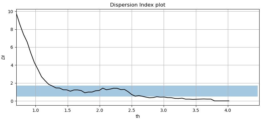
We can see that we can assume that our process is Poisson distributed with \(th \in [1.3, 2.6]\) for our selected \(dl = 48h\). Note that the plot would change if we modify the value of \(dl\). Therefore, our parameters of \(th = 2.5m \ and \ dl=48h\) are reasonable according to \(DI\) plot.
Let’s code it!#
Pseudo code is presented. Note that here the first element in a vector corresponds to index 1.
read observations

#define parameters
dl = 48 #in hours
th = linspace(min_threshold, max_threshold, step) #range_thresholds

for i in length(th):
    excesses = find_peaks(observations, threshold = th[i], distance = dl) - th[i]
    for j in length(years):
        n_excesses[j] = count(excesses[j])
    e_mean[i] = mean(n_excesses)
    var_mean[i] = var(n_excesses)

plot(x = th, y = e_mean/var_mean)