
1. Reliability Analysis Introduction#
Homework 1: start in Week 1, complete at the end of Week 3.
This assignment is meant to introduce you to the reliability calculations that make up the foundation of the unit, as well as review some fundamental concepts from MUDE (parametric distributions, Monte Carlo simulation). There are nine “questions” for you to answer, along with a few discussion questions to consider at the end. The notebook introduces a simple example and also provides code to help you through the required calculations.
Note
This page is generated from an *.ipynb file and is accompanied by an image file, all of which can be downloaded using the link below.
First, let’s get the Python package imports out of the way:
import numpy as np
import matplotlib.pyplot as plt
import pandas as pd
import scipy.stats as st
import matplotlib.cm as cm
Introduction#
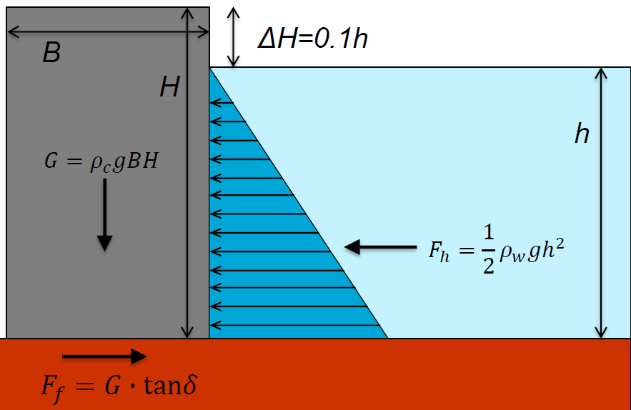
The example discussed in this homework assignment is similar to the one presented in the first lecture of Week 2 of your HOS Hydrauli Structures unit in Q3.

In the example from Q3, a “fully” probabilistic approach consisted of determining the probability of the actions (loads) being higher than the resistance (\(F_h > F_f\)). This assignment uses a more universal notation: actions (or stresses) are noted \(S\) and the resistance is noted \(R\).
Here, both \(R\) and \(S\) will follow lognormal distributions. Similarly to the notations adopted in ADK, we have \( R \sim \mathcal{LN(\lambda_R, \zeta_R)}\) and \(S \sim \mathcal{LN(\lambda_S, \zeta_S)}\).
The means and standard deviations of the random variables have already been determined from observations and are given below:
To prepare the notebook for making calculations with code, we also define the statistics (including correlation coefficient) in the following cell:
# Mean and standard deviation: R
mu_r = 8.76e5          # Mean
sigma_r = 1.41e5       # Standard deviation
cov_r = sigma_r/mu_r   # Coefficient of variation

# Mean and standard deviation: S
mu_s = 4.95e5
sigma_s = 9.89e4
cov_s = sigma_s/mu_s

rho_rs = 0.1           # Correlation coefficient between R and S
Our objective is to build a lognormal distribution to model the random variables, and it turns out and easy way of working with random variables is to store them as ‘objects’. This allows us to access the statistics or parameters of each random variable (object) with easy. The class below allows you to create a Random_Variable instance which follows a Lognormal distribution. Give it a look (it’s a few cells below) to understand how it’s built!
The class Random_Variable is presented a few cells below because first we need you help us define a few methods (functions) first. The method distrib_parameters computes the distribution parameters \((\lambda, \zeta)\) from the mean and standard deviation of the random variable \((\mu, \sigma)\).
Question 1: fill in the blank in the distrib_parameters function to test your understanding of the relation between the distribution parameters and the mean/std!
def distrib_parameters(mean, std):     # Should be left blank and filled in by students
    ''' Computes the lognormal distribution parameters.
    ---------------------------
    mean: float. Mean of the distribution.
    std: float. Standard deviation of the distribution.

    returns:
    lam: float. First distribution parameter (mean of ln(X)).
    zeta: float. Second distribution parameter (std of ln(X)).
    '''

    # Blank

    return lam, zeta
To make sure that your results in the upcoming questions are sensible, you can run the function below to test your function’s output.
def test_distrib_parameters(tolerance=1e-3):
    ''' Test function for distrib_parameters function. '''

    test_1 = distrib_parameters(8.76e5, 1.41e5)
    assert abs(test_1[0] - 13.6703) < tolerance, "Incorrect lambda value"
    assert abs(test_1[1] - 0.1599) < tolerance, "Incorrect zeta value"

    test_2 = distrib_parameters(4.95e5, 9.89e4)
    assert abs(test_2[0] - 13.0927) < tolerance, "Incorrect lambda value"
    assert abs(test_2[1] - 0.1978) < tolerance, "Incorrect zeta value"
    return None
Now we can run the cell below to define our Random_Variable class and use it!
class Random_Variable():
    ''' Create a random variable object following a Lognormal distribution.
    ---------------------------
    Parameters:
    mean: float. Mean of the distribution (X, not ln(X))
    std: float. Standard deviation of the distribution (X, not ln(X))
    '''
    def __init__(self, mean, std):
        self.mean = mean
        self.std = std
        param = distrib_parameters(mean, std)
        self.lamda = param[0]
        self.zeta = param[1]

    def change_parameters(self, mean=None, std=None):
        ''' Change the mean, standard deviation of the distribution (or both).

        mean: float. Mean of the distribution (default: None).
        std: float. Standard deviation of the distribution (default: None).
        '''
        if mean is not None:
            self.mean = mean
        if std is not None:
            self.std = std

        param = distrib_parameters(mean, std)   # Update distribution parameters
        self.lamda = param[0]
        self.zeta = param[1]

    def getDistributionParameters(self):
        return self.lamda, self.zeta

    def pdf(self, x):
        ''' Probability Density Function.

        x: float. Value at which the PDF is evaluated.
        return: PDF evaluated in x.
        '''
        zeta = self.zeta
        lam = self.lamda
        return 1/(np.sqrt(2*np.pi)*zeta*x) * np.exp(-0.5*((np.log(x)-lam)/zeta)**2)
Question 2: Use the Random_Variable class, you can create two RV objects:
# R =
# S =
Question 3: Compute the correlation coefficient \(\rho_{lnRlnS}\) between \(ln(R)\) and \(ln(S)\) (which will prove useful later on):
# rho_ln_rs =
Reliability problem formulation#
As mentioned above, the case considered here echoes the one presented in the HOS Hydraulic Structures unit from Q3. The formulation adopted then was the safety margin: we compute the probability of \(Z<0\) with \(Z = R - S\) (thus margin).
Here, the safety factor formulation is chosen as it is handier with lognormal distribution - as you’ll see later.
Question 4: define the limit state function and the associated failure event.
Hint: to read more about the safety factor formulation, see ADK 4.2.4.
Analytic Solution#
A major advantage of using the safety factor formulation in combination with lognormal distributions is the possibility to solve the problem - i.e determine the system’s failure probability - analytically.
Question 5: compute the failure probability for the distributions and dependence structure presented previously.
Hint: try to fall back on a case you know, for example normal distributions.
Monte Carlo Simulation#
A second method for solving the case is by implementing Monte Carlo Simulation.
Question 6: implement Monte Carlo analysis to check your answer numerically from Question 5. You should write the code from scratch.
Hint: you can sample both random variables using np.random.multivariate, although you might want to check the documentation to see what inputs are required. You don’t need more than 3 lines of code to solve this provlem in a reasonable way.
montecarlosize = 10000

# enter your code here

# Failure probability obtained using Monte Carlo
# pf_mc =
Question 7: check your answers from Q5 and Q6—are they the same? If not, why?
Exploring Dependence#
We will look at the bivariate PDF of \(R\) and \(S\) to explore how dependence might influence that calculated failure probability for this simple component. A good way to visualize this is by plotting contours of probability density and looking at the location of the limit state function. To do this, we need the bivariate lognormal distribution’s PDF, which is defined by:
\( f_{X,Y}(x,y) = \frac{1}{2\pi xy \zeta_x \zeta_y \sqrt{1-\rho^2}} exp \{-\frac{1}{2(1-\rho^2)}[ (\frac{ln(x) - \lambda_x}{\zeta_x})^2 + (\frac{ln(y) - \lambda_y}{\zeta_y})^2 - 2\rho(\frac{ln(x) - \lambda_x}{\zeta_x})(\frac{ln(y) - \lambda_y}{\zeta_y})]\} \)
Question 8: implement the bivariate lognormal PDF in the Python function outlined below.
def bivariate_LN(R, S, rho, r, s):
    ''' Bivariate lognormal probability density function: general case.

    R, S: Random_Variable objects.
    rho: float. Correlation coefficient between ln(R) and ln(S) (or R and S, depending on preference).
    r, s: float. Values at which the PDF is evaluated.

    returns
    pdf: probability of the event R=r and S=s.
    '''

    # Blank

    return pdf
Bivariate PDF contours#
The function below plots several interesting items, including the Limit State Function in the (R,S) plane and the bivariate PDF’s contours.
However the code is incomplete: it should also display the points generated during the Monte Carlo Simulation which correspond to the failure event (i.e \(R<S\)).
Question 9: add a few lines to the code to plot the failure realizations from your random sample in the MSC above (Q6).
def problem_plot(bivar, xlim=None, ylim=None, nb_points=200):
    """
    Contour plot in the bivariate plane (R,S).
    ---------------------
    bivar: bivariate distribution.
    xlim, ylim: tuple, list. Intervals of values of x and y displayed in the figure (default: None).
    nb_points: int. Size of the grid (default: 200).

    returns: matplotlib.pyplot Figure and Axis objects.
    """
    f, ax = plt.subplots(1)

    if xlim is None:
         xlim = [R.mean - 3*R.std, R.mean + 3*R.std]
    if ylim is None:
         ylim = [S.mean - 3*S.std, S.mean + 3*S.std]

    x = np.linspace(xlim[0], xlim[1], nb_points)
    y = np.linspace(ylim[0], ylim[1], nb_points)
    X,Y = np.meshgrid(x,y)
    pdf = np.zeros(X.shape)
    for i in range(X.shape[0]):
            for j in range(X.shape[1]):
                if X[i,j]>0 and Y[i,j]>0:
                    pdf[i,j] = bivar(R, S, rho_ln_rs, X[i,j], Y[i,j])

    ax.contour(X, Y, pdf, levels=8, cmap=cm.Blues)    # plot bivariate PDF contours
    ax.plot(x, x, label='LSF', color='k')             # plot LSF
    ax.fill_between(x, x, ylim[1], label='Failure domain', color='grey')   # fill failure domain

    # We want to extract MC realisations of failure
    # Blank

    # Plot the data obtained above
    # ax.scatter(?, ?,  label='MCS', color='k', marker='+')

    ax.set_aspect("equal")
    ax.set_xlim(xlim)
    ax.set_ylim(ylim)
    ax.set_xlabel(r"$R$")
    ax.set_ylabel(r"$S$")
    ax.legend()
    return f, ax
Once the code cell above is complete, you can generate the plot as follows:
f, ax = problem_plot(bivariate_LN)
You can find several objects on the figure above.
The grey area corresponds to the failure domain, that is the region for which \(R < S\). The black dots displayed in this region are the realisations simulated in your manual implementation of the Monte Carlso Simulation that correspond to a failure event. Finally, the blue concentric circular shapes correspond to the contours of the bivariate lognormal PDF you implemented in the previous question. Each point on the same ‘level’ (or circle) has the same density, that is the same likelihood of occurence.
Although the problem we considered was very simple, it represents one of the key types of analyses we will learn to use in this unit: a structural reliability calculation. We define a function of random variables and a failure condition (the limit-state function) and integrate over the failure domain to obtain the failure probability. Unfortunately, most of the problems we are interested in can’t be solved analytically. In fact, when the limit-state function is computationally expensive to run (e.g., a finite element program), even Monte Carlo simulation because unfeasible.
We will learn more about these methods in Week 4. For now, try thinking about the following questions and discussing them with your classmates:
What would happen if one of the random variables did not have the lognormal distribution?
How would the analytic calculation change?
What would be different in the Monte Carlo simulation?
How would the probability density contours change?
What would happen in the analysis if the limit-state function were non-linear?
How would this influence your analytic calculation?
How would this look in the bivariate plot?
What would be the effect on the calculated failure probability?
How would a different type dependence influence the result? You can check your intuition by playing with the code in this notebook!