3.2. GPD: Introduction#
After sampling the extreme observations in our time series using POT (we’ll talk more about it later), we have a sequence of independent and identically distributed excesses. Now, we want to model their statistical behavior.
Let \(F_{th}\) be the distribution function of the excesses over a threshold, \(th\),
\( F_{th} = P[X-th \leq x|X>th], \hspace{0.5cm} x \geq 0 \)
Let the excesses be \(Y=X-th\) for \(X>th\) for a sequence of \(n\) independent random variables \(X = X_1,...,X_n\).
We already saw that given:
A sequence of independent random variables \(X = X_1,...,X_n\),
The maxima of the sequence \(M_n = max(X_1,..., X_n)\), where \(n\) is the number of observations in a given block,
\(M_n\) are independent and identically distributed.
For large \(n\) the cumulative distribution function of those maxima tend to the Generalized Extreme Value (\(G(x)\), GEV) family of distributions, regardless the distribution of \(X\). If that is true, the distribution of the excesses can be approximated by a Generalized Pareto distribution [1].
Definition and parameters of GPD distribution#
The Generalized Pareto distribution is defined as
\( H(y) = \left\{ \begin{array}{ll} 1 - \left(1+\frac{\xi y}{\sigma_{th}}\right)^{-1/\xi} \hspace{1cm} for \ \xi \neq 0\\ 1 - exp\left(-\frac{y}{\sigma_{th}}\right)\hspace{1.3cm} for \ \xi = 0 \end{array} \right. \)
where \(y\geq0\) if \(\xi \geq 0\), and \(0\leq y\leq -\frac{\sigma_{th}}{\xi}\) if \(\xi<0\).
When applied to model the excesses over a threshold, we are calculating conditional probabilities to \(X>th\). This distribution function can be computed as function of the random variable \(X\) and the threshold \(th\) as
\( P[X<x|X>th] = \left\{ \begin{array}{ll} 1 - \left(1+\frac{\xi (x-th)}{\sigma_{th}}\right)^{-1/\xi} \hspace{1cm} for \ \xi \neq 0\\ 1 - exp\left(-\frac{x-th}{\sigma_{th}}\right)\hspace{1.6cm} for \ \xi = 0 \end{array} \right. \)
If our previous assumption holds, the parameters of the GPD can be determined based on those of the GEV: the shape parameter (\(\xi\)) is the same for both distributions, and \(\sigma_{th}\) is function of the location and scale parameters of the GEV as
\( \sigma_{th} = \sigma + \xi (th-\mu) \)
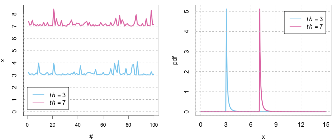
Note that \(th\) acts like a location parameter for the GPD distribution. In the plot below, this effect is illustrated.
Similarly to the GEV, \(\xi\) determines the behavior of the tail of the distribution. If \(\xi<0\), the distribution presents an upper bound at \(th-\sigma_{th}/\xi\). If \(\xi>0\), the distribution has a heavy upper tail that behaves like a power function of the exponent \(-1/\xi\). If both \(\xi=0\) and \(th=0\), GPD reduces to the Exponential distribution and if \(\xi=-1\), to the uniform distribution. We can see it in the following plot.
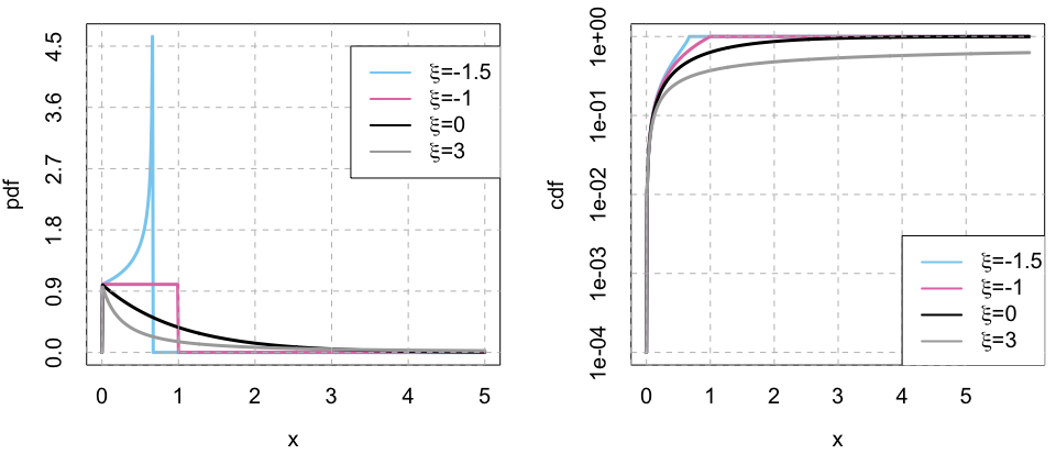
In the above plot, we have the cdf of four GPDs with a \(th=0\), \(\sigma_{th}=1\) and \(\xi=-1.5, \ -1, \ 0 \ and \ 3\). We can see the cdfs of the GPD with \(\xi=-1.5 \ and \ -1\) have a clear upper bound in \(x=0.67 \ and \ 1\), respectively. If we apply the previous formula \(th-\sigma_{th}/\xi = 0-1/(-1.5)=0.67\) and \(0-1/(-1)=1\), which fit our visual observation.
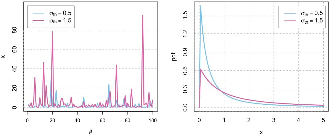
Regarding the scale parameter \(\sigma_{th}\), it presents a behavior equivalent to that observed on \(\sigma\) for the GEV distribution. The higher \(\sigma_{th}\), the wider the pdf of the distribution.