Minimal concepts of graph theory#
Vines and Bayesian Networks (BNs) combine graph theory with probability theory. For this reason we introduce minimal concepts of graph theory.
Because of his discussion of a famous problem called the Konigsberg bridge problem, Leonhard Euler is acknowledged as the father of graph theory. This problem appears in almost any modern text book on graph theory. Euler’s original paper is written in Latin, for a translation to English the reader is referred to Biggs et al. (1986)[1]. Like many problems in probability theory, some of the early developments of graph theory originated from games. One of these was the hamiltonian game invented by Sir William Hamilton. The hamiltonian game will be used to introduce some definitions and notation that will be used later in the rest of the thesis.
An undirected graph \(G = (N,E)\) consists of a finite non empty set \(N\) of nodes, also called (points or vertices) and a possibly empty set \(E\) of edges (lines or arcs) where each element is an unordered pair \((\alpha_1,\alpha_2)\), where \(\alpha_1\) and \(\alpha_2 \neq \alpha_1\) are elements of \(N\). Without loss of generality, when \(N =\{1,2,...,n\}\) we speak of labeled graphs. It will be assumed that two distinct edges do not join the same pair of nodes. Graphs in which this is allowed are called multigraphs. Observe that no self-loops are permitted that is, edges joining nodes with itself. If the pair \((\alpha_1,\alpha_2)\) is ordered then \(G\) is a directed graph and the pair \((\alpha_1,\alpha_2)\) will be represented as \(\alpha_1 \rightarrow \alpha_2\). In this case \(\alpha_1\) will be called a parent node of the child node \(\alpha_2\). Examples of undirected and directed graphs are shown in the Figures below.
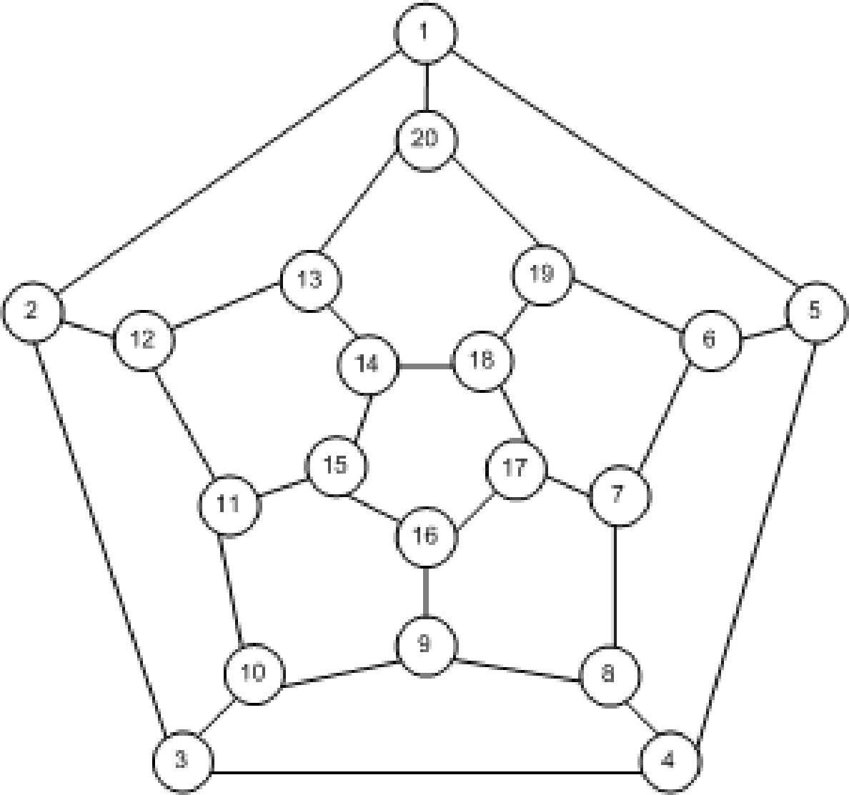
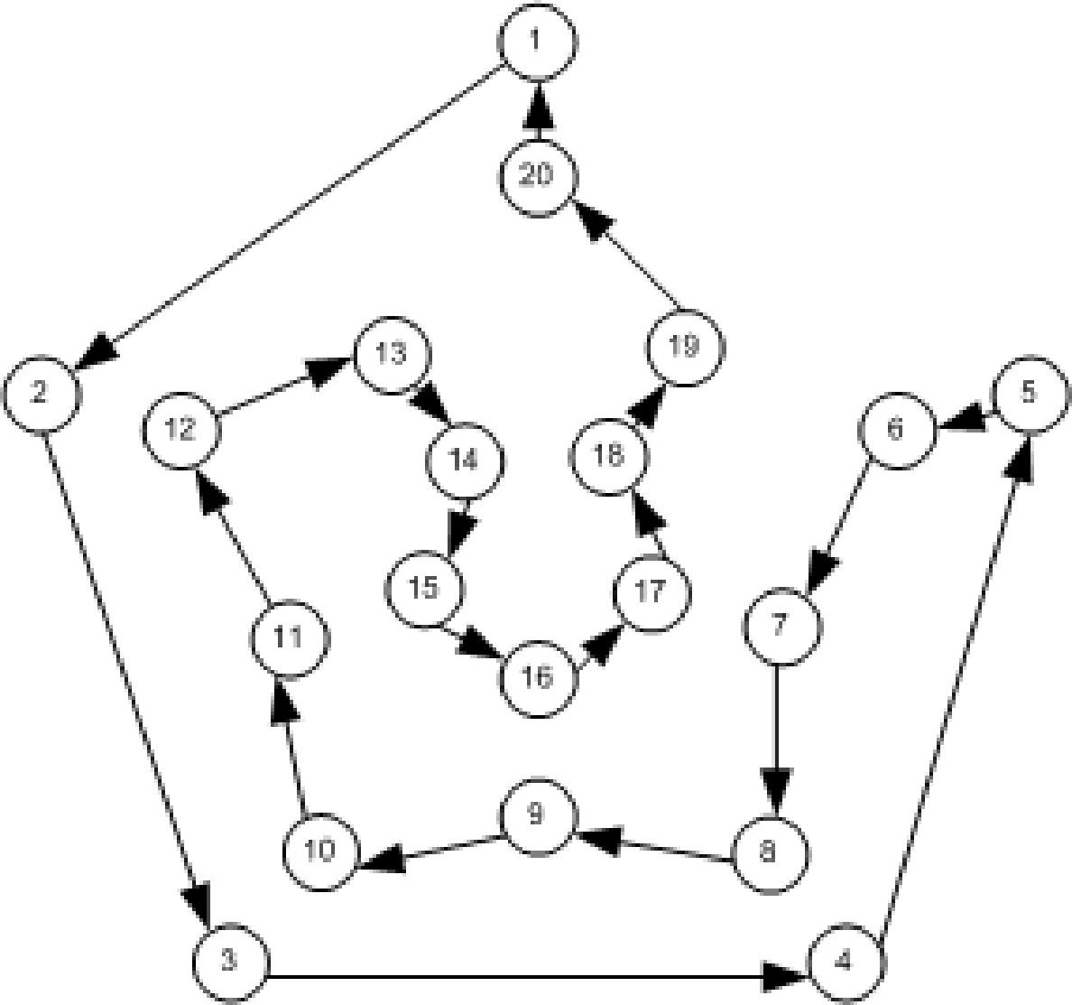
Figure 1. Examples of graphs: (left) undirected, and (right) directed.
The cardinality of \(N\) is called the order of the graph. If the pair \((\alpha_1,\alpha_2) \in E\) then the two nodes \(\alpha_1\) and \(\alpha_2\) are adjacent and each one is incident with the pair \((\alpha_1,\alpha_2) \in E\). The degree of a node is the number of edges incident with it. A complete graph \(CG\) has every node adjacent to each other. A path of length \(n\) from \(\alpha\) to \(\beta\) is a sequence \(\alpha= \alpha_0, . . . , \alpha_n = \beta\) of distinct nodes such that \((\alpha_{i-1}, \alpha_{i}) \in E\) for all \(i = 1, . . . , n\). A cycle is a path such that \(\alpha = \beta\). If every pair \((\alpha_{i-1}, \alpha_{i})\) in a cycle of a directed graph is ordered as in \(E\) then it is a directed cycle otherwise it is an undirected cycle. If a directed graph has no directed cycles, then it is a directed acyclic graph (DAG).
Hamilton proposed a graph like the one in Figure 1 where each node represented a city of the world and the edges connections between the cities. The object of the game was to travel “Around the World” by finding a route that passes through each node exactly once. In other words, the object of the game was to find a cycle of the graph in Figure 1 such that all nodes in \(N\) are contained in the cycle. One possible such cycle is represented by the directed graph in Figure 1(right). According to Harary (1967)[2] “Hamilton sold this idea to a game manufacturer in Dublin for about twenty-five guineas which was wise of him since it was not a commercial success”.[3]
Since the introduction of graphs by Euler, its applications to many fields of science has grown. Probability theory has also relied on graphs to advance its methods. Two types of graphs will be of special importance in this course: directed acyclic graphs and trees. A tree is a graph without cycles. Notice that trees can be directed or non-directed.