Bayesian filters

Fundamentally, all data assimilation (DA) algorithms leverage Bayes’ Theorem. Before we dive into the methodological details, we should first establish some necessary vocabulary. In data assimilation, we usually care about the inference of states and/or parameters by assimilating observations:

• states are (typically) time-varying uncertain quantities of interest; typical examples of states would be quantities like soil moisture, temperature, wave height, stock price, blood pressure, or mechanical load. In this chapter, we will refer to states with the variable \(\boldsymbol{x}\).

• parameters are (typically) time-invariable uncertain quantities of interest; typical examples include the gravitational constant, the porosity of a subsurface medium, the geometry of a dike, or the volatility in a certain stock price. In this chapter, we will refer to parameters with the variable \(\boldsymbol{\theta}\).

• observations are properties of a system that we can measure or observe. These can be observations of states, parameters, or any combination thereof. In this chapter, we will refer to observations with the variable \(\boldsymbol{y}^{*}\).

Data assimilation further requires two important pieces - a forecast model and an observation model:

• a forecast model is a conventional numerical or analytical model that predicts quantities of interests (states or parameters) based on other quantities of interest (states or parameters). From a statistical perspective, these models establish a statistical relationship between the states \(\boldsymbol{x}\) and/or the parameters \(\boldsymbol{\theta}\).

• an observation model relates these quantities of interest to our observations \(\boldsymbol{y}^{*}\) by making observation predictions \(\boldsymbol{y}\). From a statistical perspective, observation models establish a statistical relationship between the states \(\boldsymbol{x}\) and parameters \(\boldsymbol{\theta}\) with the observation predictions \(\boldsymbol{y}\).

In broader literature, there are different types of DA algorithms which vary in scope and approach. The most common examples are:

• Variational DA: These methods seek to identify a maximum a posteriori estimate of the states and parameters, that is to say, the most probable combination of states and parameters. As such, they usually do not provide uncertainty estimates.

• Bayesian smoothers seek to infer the full posterior of the states and parameters \(p(\boldsymbol{x}_{1:T},\boldsymbol{\theta}|\boldsymbol{y}_{1:T}^{*})\), that is to say, the best possible estimate of our quantities of interest. Example applications include subsurface reservoir characterization or forensic analysis.

• Bayesian filters only seek to infer the posterior of the latest states \(p(\boldsymbol{x}_{T},\boldsymbol{\theta}|\boldsymbol{y}_{1:T}^{*})\) given all information so far. This makes filters very useful in systems in which we want to know the latest state, but do not necessarily care about improving hindsight. Example applications include stock trading, robotics, tracking, weather forecasting, or pump control.

In this chapter, we will focus only on Bayesian filters. However, much of the methodology can be applied directly to Bayesian smoothing applications, as well!

A brief recapitulation of Bayes’ Theorem

As established, Bayes’ Theorem lies at the heart of DA. To begin, let us recall the basic principles of Bayesian inference. Assuming that we have two random variables \(\boldsymbol{x}\) and \(\boldsymbol{y}\) (ignoring parameters for the time being), Bayes’ Theorem is defined as:

\[ \underbrace{p(\boldsymbol{x}|\boldsymbol{y}^{*})}_{\text{posterior}} = \frac{p(\boldsymbol{y}^{*},\boldsymbol{x})}{p(\boldsymbol{y}^{*})} = \frac{\overbrace{p(\boldsymbol{x})}^{\text{prior}}\overbrace{p(\boldsymbol{y}^{*}|\boldsymbol{x})}^{\text{likelihood}}}{\underbrace{p(\boldsymbol{y}^{*})}_{\text{model evidence}}} \]

There are two separate things happening here:

1. We combine the prior \(p(\boldsymbol{x})\) and the observation model \(p(\boldsymbol{y}|\boldsymbol{x})\) into a joint probability distribution \(p(\boldsymbol{x},\boldsymbol{y})\) between the states \(\boldsymbol{x}\) and observation predictions \(\boldsymbol{y}\). Mind that the observation model yields a likelihood \(p(\boldsymbol{y}^{*}|\boldsymbol{x})\) once we plug in a specific observation value \(\boldsymbol{y}^{*}\).

2. We then condition this joint distribution \(p(\boldsymbol{x},\boldsymbol{y})\) on a specific observation value \(\boldsymbol{y}^{*}\) to obtain the posterior distribution \(p(\boldsymbol{x}|\boldsymbol{y}^{*})\).

A discrete example: profiling a bank robber

Assume that you are tasked with assembling a physical description of a bank robber. Since the bank robber was wearing a mask, we have conflicting information about his hair color \(x\) - the witnesses cannot agree what his hair color was. Most of them think his hair color was brown (49%), some of them claimed it was blond (22%), and a few thought it was black (18%) or red (11%). This allows us to define a prior distribution \(p(x)\).

Fortunately, we caught a lucky break: the cashier was actually close enough to the bank robber to see his eye color \(y\), and she noticed that his eyes were \(y^{*}=\text{green}\). Does this help us to improve our knowledge about his hair color? Yes!

As it turns out, there is a genetic link between hair color and eye color. If we know the prevalence of eye colors among people with different hair colors, we obtain the equivalent to an observation model \(p(y|x)\). Multiplying these likelihoods with the hair color probability obtained from our witnesses - the equivalent to a prior \(p(x)\) (Step 1) - we can form a contingency table that represents the probability of every conceivable combination of hair color and eye color, or a discrete joint probability distribution \(p(x,y)\) (Step 2). Conditioning on the actual eye color we have observed (\(y^{*}=\text{green}\)) then amounts to reading out the correct row of this contingency matrix, and normalizing it across the sum of probabilities in this row (the model evidence \(p(y^{*})\); Step 3).

After doing this, we obtain a posterior estimate of the bank robbers hair color: we remain confident that his hair color may have been brown (48% to 46%), have increased our belief that his hair color may have been blond (22% to 27%) or red (11% to 18%), and have halved our belief that his hair color may have been black (18% to 9%).

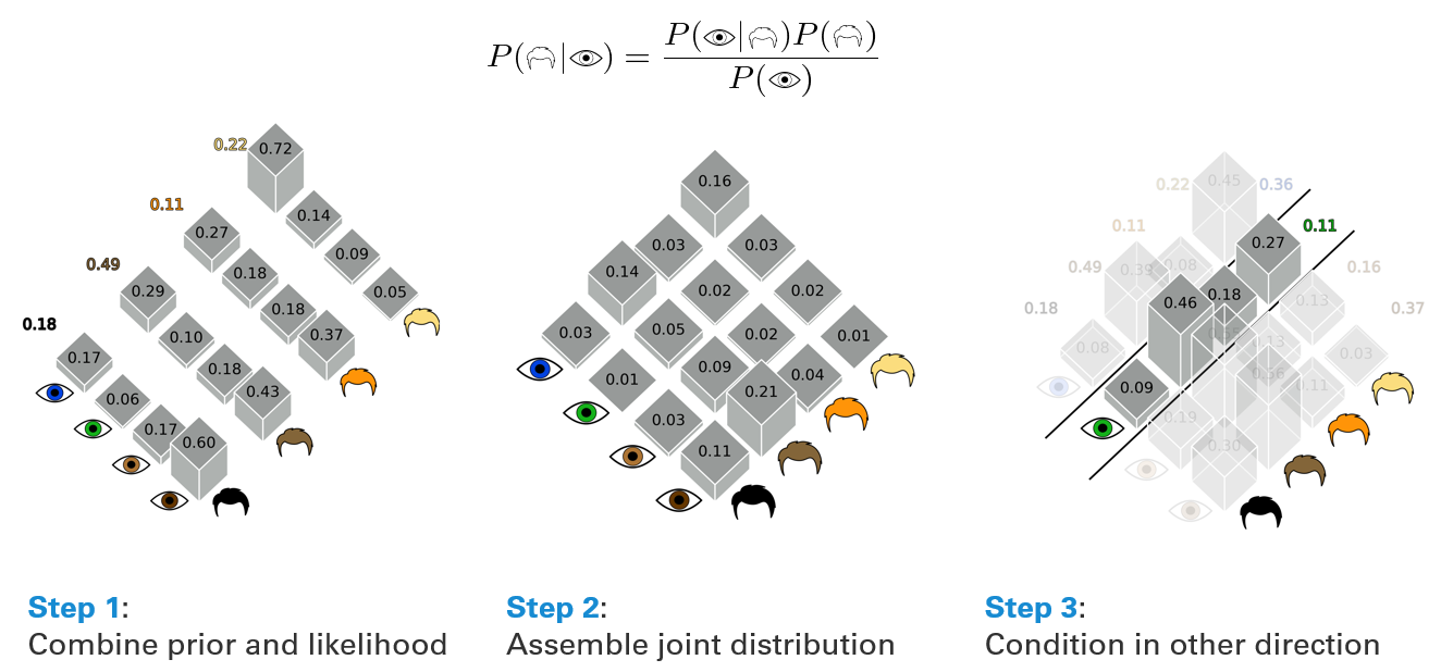
Fig. 57 How to create a contingency table for hair color and eye color, and use it to obtain posterior probabilities.

The continuous case

Most random variables we deal with are of course not discrete but continuous, which means that a contingency table would require infinitely many rows and columns. Instead, we this work with operations on probability density functions (pdfs):

• summing across rows or columns becomes marginalization, which is achieved by integrating out a variable: $\(p(\boldsymbol{y})=\int p(\boldsymbol{y},\boldsymbol{y}) d\boldsymbol{x}\)$

• conditionalization is achieved by freezing one input variable (say: \(\boldsymbol{y} := \boldsymbol{y}^{*}\)) and then normalizing against its marginal probability density \(p(\boldsymbol{y}^{*})\): $\(p(\boldsymbol{x}|\boldsymbol{y}^{*})=\frac{p(\boldsymbol{y}^{*},\boldsymbol{x})}{p(\boldsymbol{y}^{*})}\)$

While these operations are conceptually simple, their practical implementation is very difficult. In the continuous case, each of these operations requires the manipulation of functions rather than numbers. Since these PDFs have to describe the precise probability (density) of arbitrary combinations of states, parameters, and observations, the distributions they describe can be extremely complex. In practice, it is thus rarely possible to write down closed-form expressions for PDFs, which in turn makes it mpossible to manipulate them. Since we require both joint distributions, marginalization, and conditioning for Bayesian inference, this makes analytic solutions to Bayesian inference difficult.