Copula Families

In univariate analysis, we can describe data using parametric (theoretical) distribution functions or construct empirical distributions directly from observed data. The same principles extend naturally to the multivariate setting.

Parametric copula families provide flexible tools to model and describe a wide range of dependence structures among multiple variables, capturing relationships that go beyond simple correlations. At the same time, empirical copulas allow us to construct joint distributions directly from data without assuming a specific parametric form, generalizing the familiar idea of empirical distributions from the univariate case.

Together, parametric and empirical approaches form the foundation for modelling and describing dependence in multivariate data.

Empirical Copula

The empirical copula is a nonparametric estimator of the copula and provides the empirical joint distribution function of two dependent random variables.

Let us consider two dependent random variables \(X\) and \(Y\) of length \(n\), with ranks \(R_X\) and \(R_Y\), respectively. The empirical copula is defined as

\[ C_n(u_1, u_2) = \frac{1}{n} \sum_{i=1}^n \mathbf{1}\!\left( \frac{R_{X,i}}{n} \le u_1,\, \frac{R_{Y,i}}{n} \le u_2 \right). \]

Note that, similarly to the univariate empirical distribution, this is a step function in which each step corresponds to a new observation in the sample. The empirical copula converges to the true copula as \(n \to \infty\). It is also commonly used as a reference in several goodness-of-fit methods.

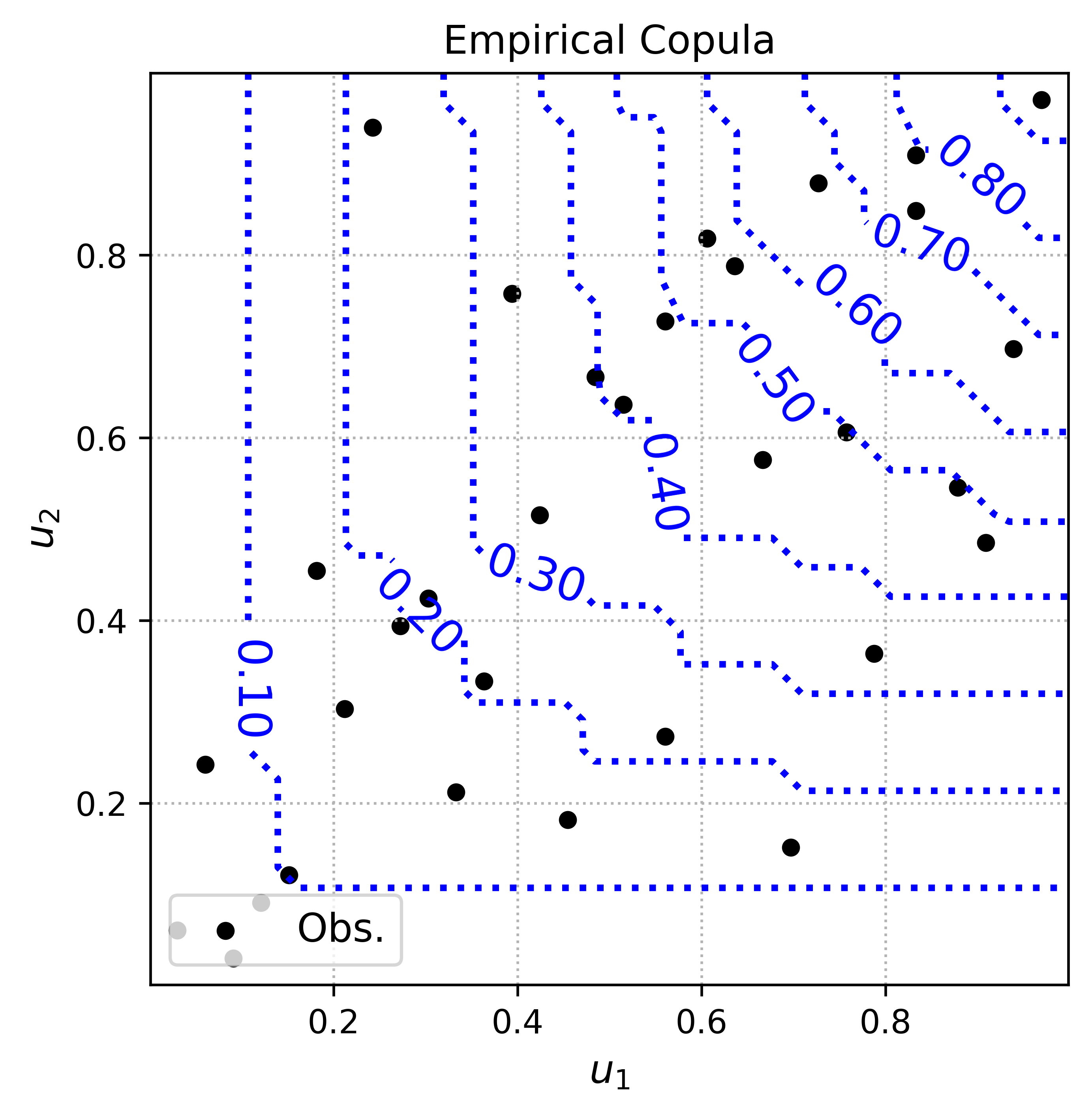
Fig. 30 The blue contour lines show the joint probability levels of the empirical copula, and the black dots correspond to the observed samples.

Theoretical Copulas

Building on the concept of empirical copulas, which provide a nonparametric representation of dependence directly from data, theoretical (or parametric) copulas allow us to describe and model multivariate dependence using a predefined functional form, in the bivariate case, a surface. Unlike empirical copulas, parametric copulas rely on a chosen family with specific properties, enabling us to capture various types of dependence patterns.

Here, we focus on three widely used one-parameter copula families that model key features of dependence, including symmetries and asymmetries, as well as stronger associations among larger or smaller values. The three families are the Gaussian copula, which is symmetric and captures linear correlation patterns; the Gumbel copula, which is asymmetric and emphasizes stronger association for larger values; and the Clayton copula, which is asymmetric and emphasizes stronger association for smaller values.

Gaussian Copulas

The Gaussian copula is an elliptical copula since it derives from Gaussian distribution which is an elliptical distribution. It models symmetric dependence structures and captures linear correlations between variables.

The bivariate Gaussian copula is constructed using a bivariate normal distribution (\(\Phi_2\)) with zero mean vector, unit variances, and Pearson’s correlation \(\rho\). More specifically,

\[ C(u_1, u_2) = \Phi_2\big( \Phi^{-1}(u_1), \Phi^{-1}(u_2); \rho \big) \]

Note that the margins follow a standard uniform distribution (\(\Phi\)). The Pearson correlation coefficient \(\rho\), which is the single parameter of the Gaussian copula, can be estimated via Kendall’s tau as

\[ \rho = \sin\Big(\frac{\tau \pi}{2}\Big). \]

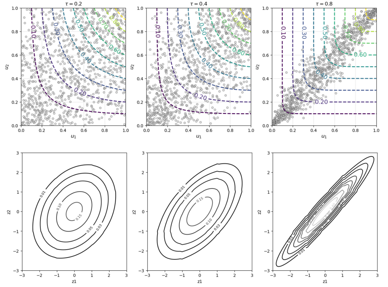
Fig. 31 CDF (top row) and PDF (bottom row) isolines for the Gaussian copula are shown for three levels of positive dependence, i.e., \(\tau = 0.2\), \(\tau = 0.4\) (middle), and \(\tau = 0.8\) (right). Note that the representations are on different scales: the CDF is in the unit space, while the PDF is in the normal space to better highlight the dependence structure.

We can see that the joint behavior and the symmetry of the Gaussian copula become more apparent as the underlying dependence between the variables increases.

Gumbel Copula

The Gumbel copula belongs to the family of Archimedean copulas. In contrast to elliptical copulas, Archimedean copulas are defined via a generator function and are capable of modeling asymmetric dependence, capturing stronger associations among larger or smaller values. For a detailed description of the generator function and Archimedean copulas in general, we refer to Czado (2019).

The Gumbel copula is defined as

\[ C(u_1,u_2) = exp[-( (-ln(u_1))^\delta + (-ln(u_2))^\delta )^\frac{1}{\delta} ] \]

where \(\delta \geq 1 \) is the copula’s parameter. For \(\delta \rightarrow \infty \) we have full dependence and for \(\delta = 1 \) we have independence. The copula’s parameter can be estimated via Kedall’s tau, as \(\delta = 1/(1-\tau)\) for \(\tau = [0,1]\) (positive dependence).

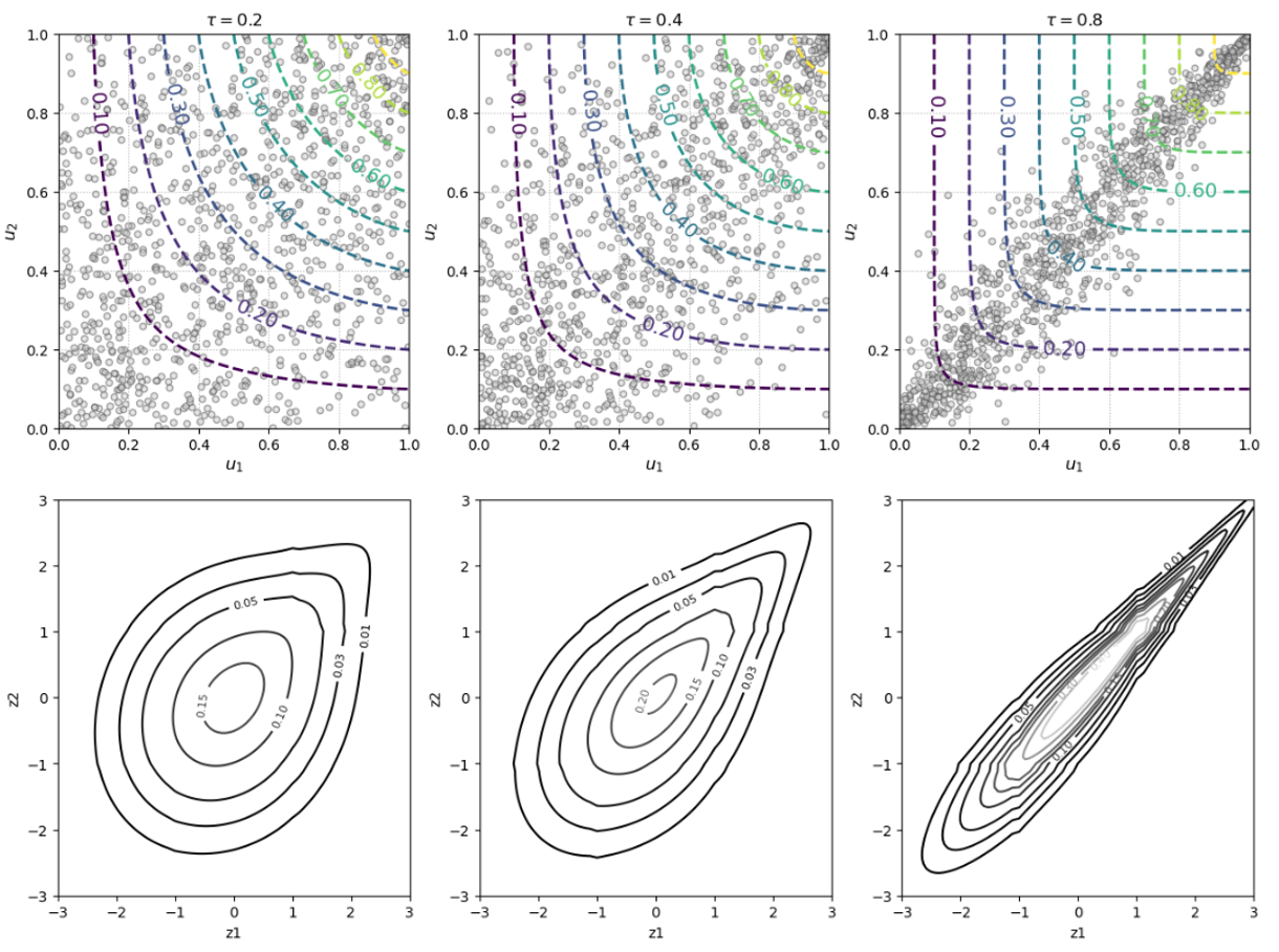
Fig. 32 CDF (top row) and PDF (bottom row) isolines for the Gumbel copula are shown for three levels of positive dependence, i.e., \(\tau = 0.2\), \(\tau = 0.4\) (middle), and \(\tau = 0.8\) (right). Note that the representations are on different scales: the CDF is in the unit space, while the PDF is in the normal space to better highlight the dependence structure.

We can see that the Gumbel copula models asymmetric dependence structures. More specifically, it captures stronger associations among larger values; this is evident from the fact that the pairs in the upper-right corner of the plots lie closer to the 1:1 line.

Clayton

The Clayton copula is also an Archimedean copula and is therefore able to model asymmetries in the dependence structure.

The Clayton copula is express as

\[ C(u_1,u_2) = (u_1^{-1} + u_2^{-1} - 1)^\frac{-1}{\delta} \]

where \(0 < \delta < \infty \) is the copula’s parameter governing the dependence. For \(\delta \rightarrow \infty \) we have full dependence, while for \(\delta \rightarrow 0 \) we have independence. The copula parameter can be estimated via the Kendall’s tau as \(\delta = \frac{2\tau}{1-\tau}\) for \(\tau = [0,1]\) (positive dependence).

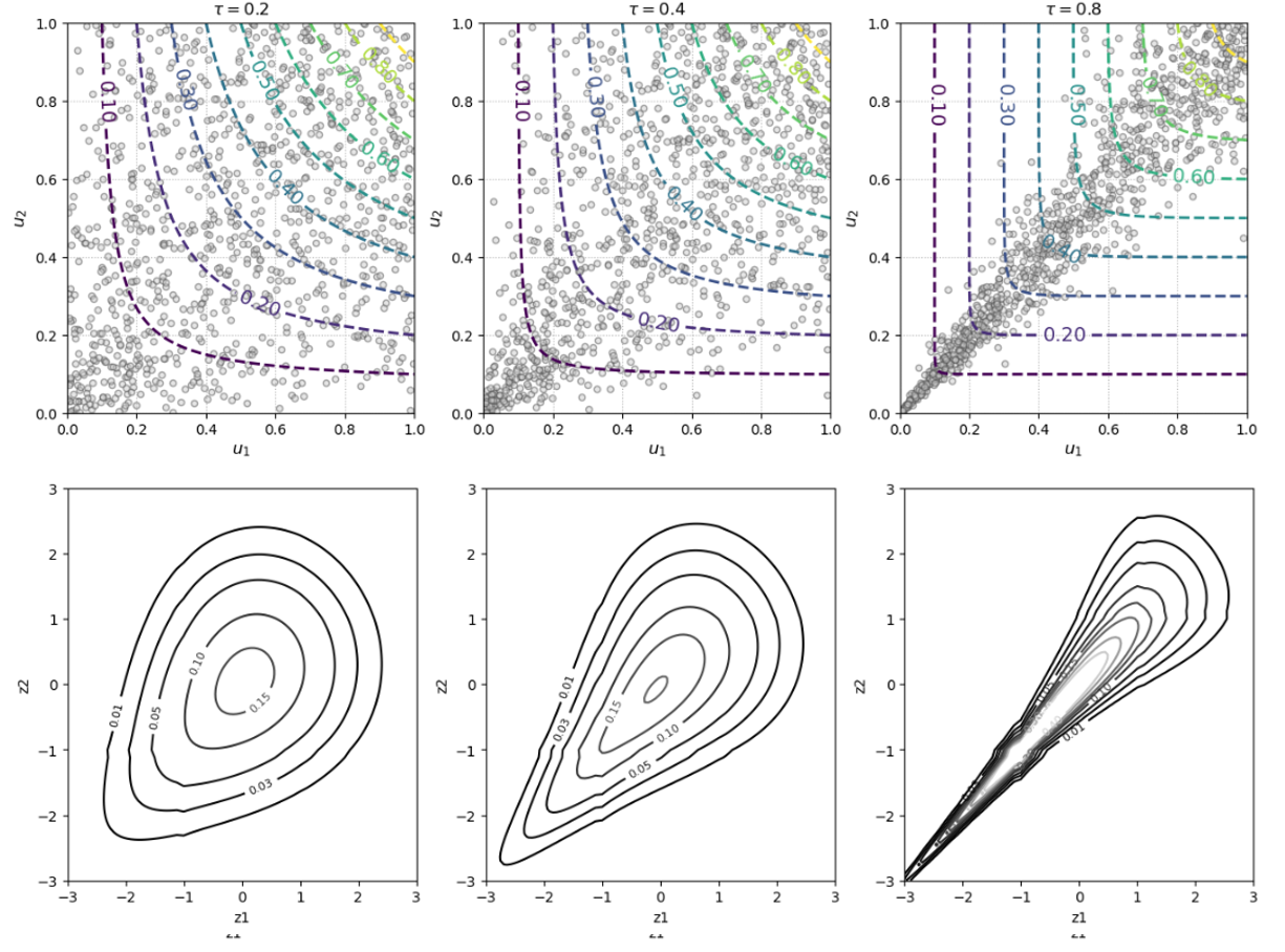
Fig. 33 CDF (top row) and PDF (bottom row) isolines for the Clayton copula are shown for three levels of positive dependence, i.e., \(\tau = 0.2\), \(\tau = 0.4\) (middle), and \(\tau = 0.8\) (right). Note that the representations are on different scales: the CDF is in the unit space, while the PDF is in the normal space to better highlight the dependence structure.

Copula Sandbox

Fig. 34 An interactive copula sandbox. Select a copula from the drop-down menu, then adjust the parameter sliders to see how it affects the copula’s probability density.

.