Bivariate Copulas#
To statistically describe dependent variables, we rely on the following components:
Marginal distributions:
\(f_X(x)\) and \(f_Y(y)\), which describe the univariate behavior of \(X\) and \(Y\), respectively.Joint density function:
\(f_{X,Y}(x,y)\), which models the joint occurrence of the pair \((X, Y)\).Conditional distributions:
\(f(x \mid y_0)\) and \(f(y \mid x_0)\), which describe the distribution of one variable (e.g., \(X\)) when conditioned on a specific value of the other (e.g., \(Y = y_0\)).
Together, these components form the foundation for analyzing and modeling multivariate dependencies (specifically bivariate), serving as a bridge between univariate analysis and more advanced multivariate statistical modeling.
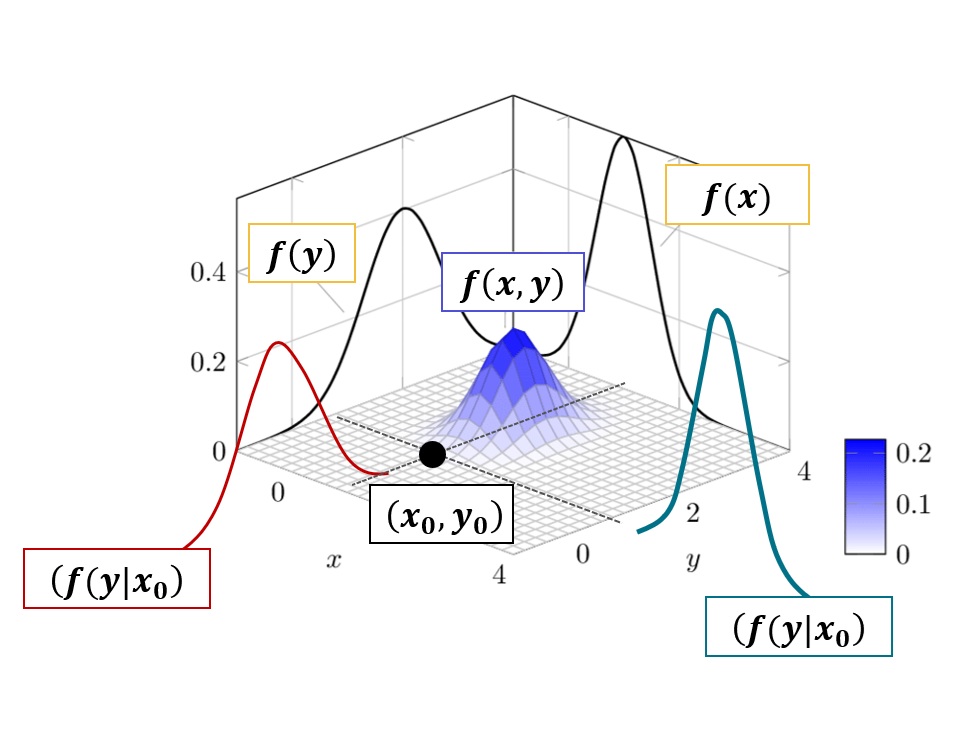
Fig. 29 Graphical representation of bivariate elements for a statistical description of dependent variables.#
We often have good knowledge of univariate distributions, such as the normal, gamma, or beta families, and these can be used to model marginal distributions (f_X(x)) and (f_Y(y)). When no suitable parametric form is available, the empirical cumulative distribution function provides a nonparametric alternative. However, specifying the marginals is only part of the task. We also want to model the joint distribution. In particular, we want a flexible way to model the joint behaviour between variables including asymmetries in their association and that is not constrained by the particular shapes or scales of the marginals.
To remove the effect of the marginals on the dependence structure, we rely on the probability integral transform (as we have seen in the previous setion), which maps each variable through its own cumulative distribution function. This produces new variables with uniform marginals on \([0,1]\), effectively removing the influence of scale and marginal behavior. What remains is the pure dependence structure, which can be modeled independently of the margins.
A copula is the tool that captures this idea. More formally, a copula is the joint distribution function of standard uniform variables. Thus, it describes the dependence between random variables free from the influence of their individual marginal distributions. In the bivariate case, a copula \(C\) is a distribution function defined on \([0,1] \times [0,1]\) with uniform marginals. If the copula is continuous, its density (c) is obtained by differentiating:
The usefulness of copulas is guaranteed by Sklar’s Theorem, which states that any multivariate distribution \(F_{X,Y}\) with marginals \(F_X\) and \(F_Y\) can be written as
Conversely, combining any copula with any pair of marginal distributions yields a valid joint distribution. This result formally separates marginal behavior from dependence and provides a flexible and powerful framework for modeling multivariate data.
Sklar’s Theorem can be extended to higher dimensions. More specifically, let \(X\) be a \(d\)-dimensional random vector with joint distribution function \(F\) and marginal distribution functions \(F_i\) for \(i = 1, \ldots, d\). Then the joint distribution function can be expressed as
with associated density or probability mass function
for some \(d\)-dimensional copula \(C\) with copula density \(c\).
For absolutely continuous distributions, the copula \(C\) is unique.
The inverse also works. The copula corresponding to a multivariate distribution function \(F\) with marginal distributions \(F_i\) for \(i = 1, \ldots, d\) can be expressed as
and its copula density or probability mass function is determined by
Dependence Measure via Copulas#
Correlation measures such as Kendall’s \(\tau\) and Spearman’s \(\rho_s\) can be expressed directly in terms of the copula, highlighting that dependence is fully captured by the copula function for continuous random variables. For a continuous pair \((X_1, X_2)\) with copula \(C\), these measures are given by
and