Return Period Under the Nonstationary Assumption

Under nonstationary conditions, the traditional definition of return period requires modification, as the statistical properties of the variable of interest change over time, or as a function of a physical covariate. Two approaches have been proposed to address this challenge: the effective return level, which adapts the return level concept to account for changes, and the expected waiting time, which focuses on the anticipated time until an event occurs. Note that the Effective Return Level is of general applicability, while the concept of Expected Waiting Time can only be used for temporal nonstationarity.

Effective Return Level.

It is often easier to understand these time trends by looking at the quantiles of the distribution, or what is called the effective return level.
If the parameters do not depend on time, this reduces to the traditional return level, i.e., the value expected to be exceeded once every \(1/p\) years, where \(p\) is the exceedance probability.

The \((1 - p)\)-th quantile of the GEV distribution, as a function of time \(t\), is obtained by inverting the cumulative distribution function:

\[ G^{-1}(1 - p \mid \mu(t), \sigma(t), \xi(t)) = \mu(t) + \frac{\sigma(t)}{\xi(t)} \left\{ [-\ln(1 - p)]^{-\xi(t)} - 1 \right\}, \quad 0 < p < 1. \]

This expression gives the value that is exceeded with probability \(p\) in a given year (or period), while allowing the parameters to vary with time.

To go back to the previous example, if the location parameter \(\mu(t)\) changes linearly over time, then the effective return level will also change linearly over time. In general, the effective return level reflects the trend in the observations.
Similarly, it is possible to evaluate the effective return level as a function of a physical covariate. For example, the location parameter may take the form \(\mu(x_c)\).

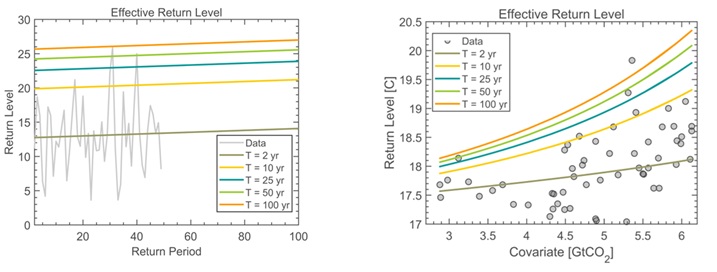
Fig. 25 Effective Return Level, i.e., isolines of constant return period (or frequency) as a function of time (left panel) and as a function of a physical covariate (right panel)

This makes it possible to interpret long-term trends in extremes, such as whether floods, heatwaves, or other extreme events are becoming more or less intense over time or as a function of a covariate.

Expected Waiting Time.

Under the assumption of nonstationarity, the distribution changes over time, and so the quantiles, as we have seen with the effective return level.

Recently, scientists and practitioners revised the concept of return period and introduced the concept of Expected Waiting Time (EWT), applicable in the case of temporal nonstationarity.

Let \(z_{q_0}\) denote the event such that \(P(Z \leq z_{q_0}) = q_0\) at time \(t_0\). Let \(p_0\) be the corresponding exceedance probability \(p_0 = 1 - q_0\). Under the assumption of nonstationarity, over time the exceedance probability of \(z_{q_0}\), which is a fixed value (for example, a design value), will change over time. More specifically, if the variable \(z\) exhibits an increasing trend over time, the event \(z_{q_0}\) will occur more often in the future since at time \(t_i > t_0\) the exceedance probability \(p_{t_1}\) is greater than the initial exceedance probability \(p_0\).

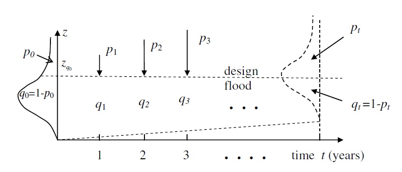
Fig. 26 Exceedance probability \(p_t\) and probability \(q_t\) changing over time. Figure 1 from Salas et al. 2014.

Let \(p_x\) be the exceedance probability at a given time \(x\) and \(x = 1,2, \cdots, x_{\max}\), where \(x_\max\) is the time at which \(p = 1 \). Note that we are treating \(x\), the time at which we evaluate the exceedance probability \(z_{q_0}\), as a random variable. The probability that \(z_{q_0}\) occurs for the first time at time \(x\) is given by

\[ f(x) = P(X=x) = p_x \prod_{t=1}^{x-1} (1 - p_t) \]

where \(f(x=1) = q_1\). This can be seen as a generalization of a geometric distribution of the time of occurrence of \(z_{q_0}\). The geometric distribution is usually implemented when modelling the number of trials up to the first success (included).

Given \(f(x)\), the return period of \(z_{q0}\), or better the expected waiting time between two consecutive events of the same magnitude can be estimated as the expectation of the time of first occurrence of \(z_{q0}\).

\[ T = E[X] = \sum_{x=1}^{x_{\max}}xf(x) = 1 + \sum_{x=1}^{x_{\max}}\prod{t=1}{x}(1-p_t) \]

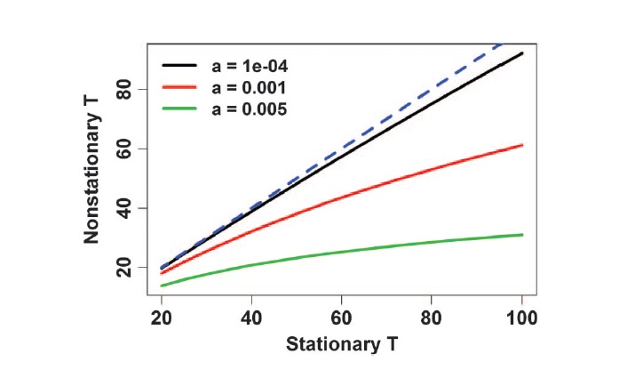
Fig. 27 Comparison between the return period under the stationary assumption and the return period estimated as EWT for different levels of trend (\(a\)) in the parameter \(\lambda\) of an exponential distribution. Figure 2 from Salas et al 2014.

For more details about EWT and its derivation, you can read Salas, Jose D., and Jayantha Obeysekera. *Revisiting the concepts of return period and risk for nonstationary hydrologic extreme events. Journal of hydrologic engineering 19.3 (2014): 554-568.