Fitting Copulas

Up to this point, we have introduced the flexibility of copulas and examined several parametric forms used to describe dependence. The next step is to put these ideas into practice. In this section, we discuss how to fit copulas to data, including the estimation of marginal distributions and the parameters governing the dependence structure.

---

In the bivariate setting, copulas are defined on the unit square domain \([0,1]^2\). Therefore, the first step in applying a copula model is to specify appropriate marginal distributions for the two variables and transform the data so that the dependence structure, separate from the marginal behavior, can be isolated and modelled via copula function.

As in the univariate case, the marginals can be estimated using either empirical distribution functions or parametric models.

Given two dependent observations \((x_{1}, x_{2})\), the transformation to the copula scale is performed via

\[ u_i = F_i(x_i), \qquad i = 1,2, \]

where \(F_i\) denotes the marginal cumulative distribution function (cdf) of \(X_i\), and \(f_i\) its probability density function (pdf).

In the case of parametric functions, the parameters of each marginal distribution can be estimated using several methods, with Maximum Likelihood Estimation (MLE) being the most common.

Let \(\theta_i\) denote the parameter vector of the chosen marginal distribution for \(X_i\). The MLE \(\hat{\theta}_i\) is defined as

\[ \hat{\theta}_i = \arg\max_{\theta_i} \, L_i(\theta_i \mid x_{i,1}, \ldots, x_{i,n}), \]

where the likelihood for the \(i\)-th margin is

\[ L_i(\theta_i \mid x_{i,1}, \ldots, x_{i,n}) = \prod_{j=1}^{n} f_i(x_{i,j} \mid \theta_i). \]

---

If the empirical distribution function is used instead of a parametric model, the transformation is performed via normalized ranks.
For each variable \(X_i\), for \(i = 1, 2\), the transfromation is computed as

\[ u_{i,j} = \frac{R_{i,j}}{n+1}, \qquad j = 1,\ldots,n, \]

where \(R_{i,j}\) is the rank of \(x_{i,j}\) among \((x_{i,1}, \ldots, x_{i,n})\). This approach avoids explicit parametric assumptions and is widely used in semi-parametric copula estimation.

---

After fitting the marginals and transforming the observations to the unit interval, \((u_{1,j}, u_{2,j})\) for \(j=1,\ldots,n\) can be used to estimate the copula model independently of the marginal specifications.

---

Fitting a copula works in a way analogous to fitting univariate distributions. Once the observations are transformed into uniform margins, and therefore lie in the copula domain, the likelihood function of the copula can be computed directly from the copula density \(c\).

For a bivariate copula \(C(u_1, u_2 \mid \delta)\) with parameter \(\delta\), the corresponding copula density is

\[ c(u_1, u_2 \mid \delta) = \frac{\partial^2}{\partial u_1\, \partial u_2} \, C(u_1, u_2 \mid \delta). \]

Given \((u_{1,j}, u_{2,j})\) for \(j = 1, \ldots, n\), the likelihood function of the copula is

\[ L(\delta) = \prod_{j=1}^{n} c(u_{1,j}, u_{2,j} \mid \delta), \]

and the maximum likelihood estimator (MLE) of the copula parameter is

\[ \hat{\delta} = \arg\max_{\delta} \, L(\delta). \]

---

For many common bivariate copula families, there exists an analytical relationship between Kendall’s \(\tau\) and the copula parameter \(\delta\).
These relationships allow for a simple method, avoiding direct maximization of the likelihood.

This method is computationally efficient and is widely used either as an initial estimate for \(\delta\) or as a standalone estimation technique. In the table below, the relationship between Kendall’s \(\tau\) and the parameter \(\delta\) is provided for the most common one-parameter copulas introduced so far.

---

Family	Kendall’s (\tau)	Range of (\tau)
Gaussian	$\(\tau = \frac{2}{\pi}\arcsin(\rho)\)$	$\([-1, 1]\)$
t	$\(\tau = \frac{2}{\pi}\arcsin(\rho)\)$	$\([-1, 1]\)$
Gumbel	$\(\tau = 1 - \frac{1}{\delta}\)$	$\([0, 1]\)$
Clayton	$\(\tau = \frac{\delta}{\delta + 2}\)$	$\([0, 1]\)$

---

Rotated copulas

It is worth noting that for the Clayton and Gumbel copulas, the relationship between Kendall’s \(\tau\) and the parameter \(\delta\) is defined only under positive dependence. This implies that, in the presence of negative dependence, one of the margins must be rotated so that the fitting procedure can be carried out using the positive–dependence version of the copula. After the copula has been fitted, the results are then rotated back to represent the original dependence structure.

More specifically, suppose the variables \(u_1\) and \(u_2\) exhibit negative dependence. We can rotate one of the margins, for instance,

\[ \hat{u}_1 = 1 - u_1, \]

which corresponds to a \(90^\circ\) rotation. The transformed pair \((\hat{u}_1, u_2)\) will then display positive dependence, allowing us to estimate the copula parameters using the standard, non-rotated version of the model.

Once the copula has been fitted, we can compute the joint probability for \((u_{1,0}, u_{2,0})\) using the rotated copula \(C_R\). The relationship between the original copula \(C\) and the rotated version is given by

\[ C(u_{1,0}, u_{2,0}) = u_{2,0} - C_R(\hat{u}_{1,0},\, u_{2,0}), \]

where \(\hat{u}_{1,0} = 1 - u_{1,0}.\)

This transformation ensures that the fitted copula correctly reflects the negative dependence in the original data.

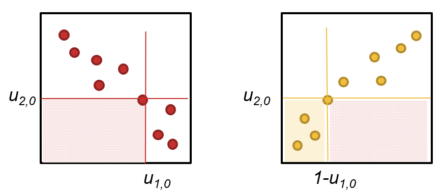
Fig. 36 Negative dependent variables (left panel, red dots). The rotation (right panel, yellow dots) allows the use of the Kendall’s \(\tau\) fitting procedure. Note that the rotated copula yields a different probability (right panel — yellow shaded area) compared to the copula in the original domain (left panel — red shaded area).

Rotation can be regarded as a powerful tool in copula applications. In general, rotations can be performed along both axes; for instance, a \(180^\circ\) rotation effectively flips the copula.

A practical application of rotation arises when the data exhibit specific asymmetries, such that a rotated version of a copula provides a better fit than the classical, non-rotated form.

For example, a \(180^\circ\) rotated Gumbel copula can be used to model stronger association between lower values, whereas the standard (non-rotated) Gumbel copula models stronger association between higher values.

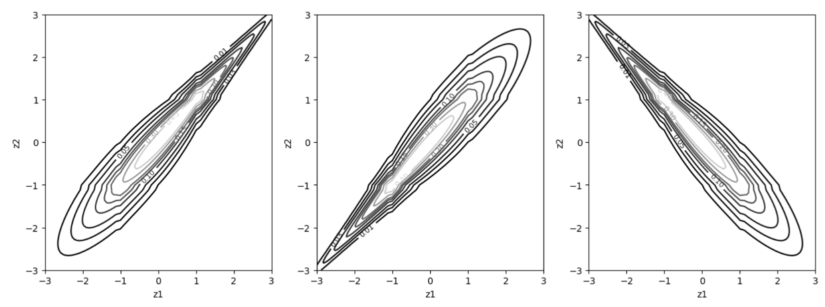
Fig. 37 Gumbel copula (left panel). \(180^\circ\) rotated Gumbel (middle panel). \(90^\circ\) rotated Gumbel (right panel). Note that the copula densities are shown with marginals on the normal scale.