Tail Dependence

Copulas are a flexible tool for modeling dependence between random variables. They allow us to investigate a wide range of dependence structures, including different levels of association and asymmetries. One concept that captures these features is tail dependence, which quantifies how the dependence between variables becomes stronger in the extremes of their distribution, even when the overall dependence (e.g., measured by Kendall’s \(\tau\)) remains constant.

Formally, tail dependence measures the probability that one variable takes an extreme value given that the other variable is also extreme. Let \(U_1 = F_1(X_1)\) and \(U_2 = F_2(X_2)\) be the marginally transformed variables on the unit interval via the probability integral transform, and let \(C(u_1, u_2)\) be their copula. The upper tail dependence coefficient \(\lambda_U\) and the lower tail dependence coefficient \(\lambda_L\) are defined as

\[ \lambda_U = \lim_{t \to 1^-} P(U_1 > t \mid U_2 > t) = \lim_{t \to 1^-} \frac{1 - 2t + C(t, t)}{1 - t}, \]

\[ \lambda_L = \lim_{t \to 0^+} P(U_1 \le t \mid U_2 \le t) = \lim_{t \to 0^+} \frac{C(t, t)}{t}. \]

In practical terms, \(\lambda_U\) and \(\lambda_L\) represent the conditional probability of observing a high (or low) value of one variable given that the other variable is also high (or low).

Based on the copulas introduced so far, the Gaussian copula does not exhibit tail dependence (both \(\lambda_U = 0\) and \(\lambda_L = 0\)), while the Clayton copula exhibits lower-tail dependence (\(\lambda_L > 0\), \(\lambda_U = 0\)) and the Gumbel copula exhibits upper-tail dependence (\(\lambda_U > 0\), \(\lambda_L = 0\)). This property makes also rotated versions of copulas particularly useful when modeling asymmetric tail behavior.

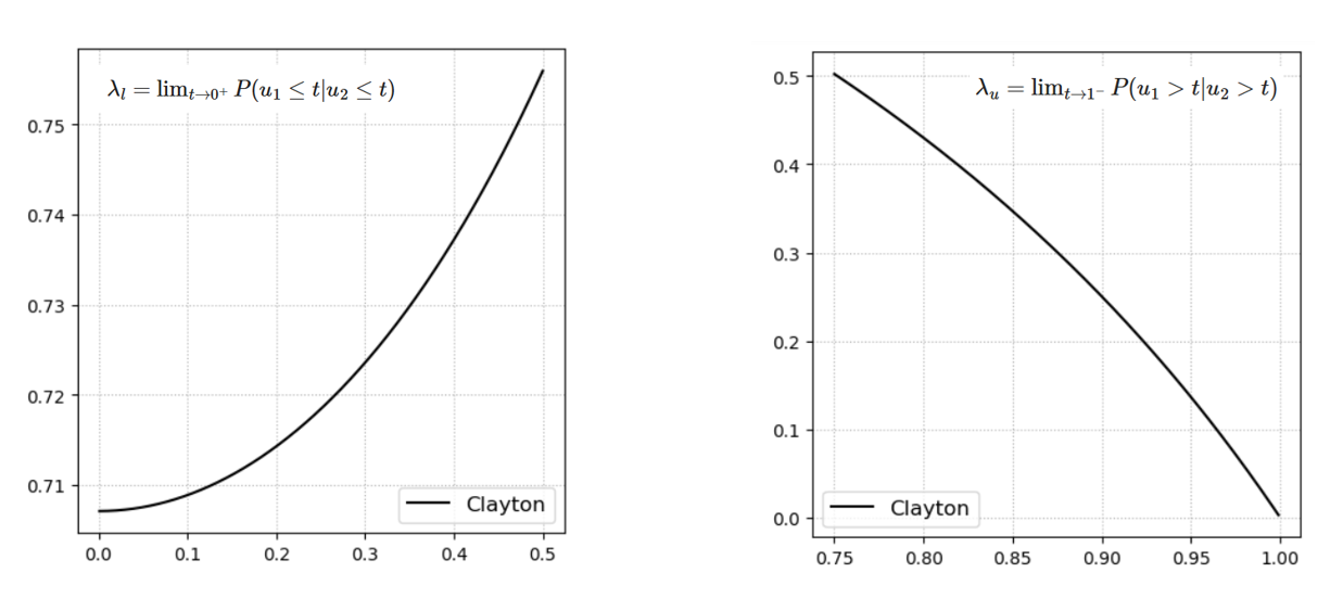
Fig. 35 Conditional probability applied to the Clayton copula to illustrate tail dependence. The left panel shows that the conditional probability remains high as values approach the lower tail (low values), while the right panel shows that it approaches zero as values move toward the upper tail (high values).

Conditional Copulas and Sampling

Through the concept of tail dependence, we have already introduced conditional probability, i.e., the probability of one variable given information about another variable.

In the context of bivariate models, and more generally in multivariate distributions, conditional probabilities are extremely useful to describe how one variable affects another. They also play a central role in inference and in sampling from a joint distribution, ensuring that the dependence between variables is preserved.

In the bivariate case, the joint density can be expressed as

\[ f(x_1, x_2) = c\big(F_1(x_1), F_2(x_2)\big) \, f_1(x_1) \, f_2(x_2), \]

where \(F_i(x_i)\) and \(f_i(x_i)\) are the marginal cumulative distribution function (cdf) and probability density function (pdf) of \(X_i\), respectively, and \(c(u_1, u_2)\) is the copula density.

Conditionalizing on one variable reduces the dimension of the probability distribution. For example, the conditional distribution of \(X_1\) given \(X_2 = x_2\) is

\[ f_{X_1|X_2}(x_1 | x_2) = \frac{f(x_1, x_2)}{f_2(x_2)} = c\big(F_1(x_1), F_2(x_2)\big) \, f_1(x_1), \]

where the effect of the dependence is captured through the copula. More generally, in higher dimensions, conditioning reduces the distribution’s dimension by the number of conditioning variables.

---

When conditional distributions are derived directly from copulas they are often called h-functions. More specifically, for a bivariate copula \(C(u_1, u_2)\), the h-function of \(U_1\) given \(U_2\) is

\[ h_{1|2} = C_{1|2}(u_1 \mid u_2) = \frac{\partial}{\partial u_2} C(u_1, u_2), \]

while the h-function of \(U_2\) given \(U_1\) is

\[ h_{2|1} = C_{2|1}(u_2 \mid u_1) = \frac{\partial}{\partial u_1} C(u_1, u_2). \]

These functions represent the conditional non-exceedance probabilities:

\[ C_{1|2}(u_1 \mid u_2) = P[U_1 \le u_1 \mid U_2 = u_2], \quad C_{2|1}(u_2 \mid u_1) = P[U_2 \le u_2 \mid U_1 = u_1]. \]

Computing Conditional Probability

Conditional probabilities in the copula domain can be computed using different approaches.

1. Empirical approach

One simple method is to use the empirical approach, counting the occurrences in the transformed domain defined by the conditioning statement. For example, the conditional probability that \(U_2\) exceeds a threshold \(u_{2,0}\) given that \(U_1\) exceeds \(u_{1,0}\) can be estimated as:

\[ P(U_2 > u_{2,0} \mid U_1 > u_{1,0}). \]

2. Using copulas and Bayes’ rule

Alternatively, conditional probabilities can be computed analytically using the copula representation combined with Bayes’ rule. In the bivariate case:

\[ P(U_2 > u_{2,0} \mid U_1 > u_{1,0}) = \frac{P(U_2 > u_{2,0}, \, U_1 > u_{1,0})}{P(U_1 > u_{1,0})}. \]

Expressing the joint probability in terms of the copula \(C(u_1, u_2)\):

\[ P(U_2 > u_{2,0}, \, U_1 > u_{1,0}) = 1 - u_{1,0} - u_{2,0} + C(u_{1,0}, u_{2,0}), \]

and since \(P(U_1 > u_{1,0}) = 1 - u_{1,0}\), the conditional probability becomes:

\[ P(U_2 > u_{2,0} \mid U_1 > u_{1,0}) = \frac{1 - u_{1,0} - u_{2,0} + C(u_{1,0}, u_{2,0})}{1 - u_{1,0}}. \]

This probabilities are easily visible in the copula space since the entire domain has unit area

Note that the probabilities in the copula domain are the same as in the original domain, according to Sklar’s theorem.”

---

Sampling from a Copula

The h-functions play a central role in copula-based sampling, as they allow us to sequentially generate dependent samples while preserving the joint dependence structure.

A standard procedure to generate dependent samples from a bivariate copula is as follows:

1. Step 1: Sample \(u_2\) from a uniform distribution \(U \sim \text{Uniform}[0,1]\).

2. Step 2: Sample \(u_1\) from the conditional copula (h-function) \(C_{1|2}(u_1 \mid u_2)\), which represents the conditional non-exceedance probability of \(U_1\) given \(U_2 = u_2\).

Sampling becomes particularly important in higher dimensions, where explicit expressions for joint probabilities are often unavailable. In such cases, sequential sampling using h-functions is a practical approach to generate dependent observations while maintaining the specified dependence structure.