Pseudo-algorithm#
With a linear observation model \(\boldsymbol{H}\), the EnKF can be implemented as follows:
Draw \(N\) samples from the prior \(\boldsymbol{X}_{1} \sim p(\boldsymbol{x}_{1})\)
For timestep \(t\) from \(1\) to \(T\):
Assimilation step
Estimate the empirical covariance
\(\boldsymbol{\Sigma}_{t} = \frac{1}{N-1}\sum_{n=1}^{N}[\boldsymbol{X}_{t}^{n} - \mathbb{E}[\boldsymbol{X}_{t}]][\boldsymbol{X}_{t}^{n} - \mathbb{E}[\boldsymbol{X}_{t}]]^\intercal\)
Compute the Kalman gain
\(\boldsymbol{K} = \boldsymbol{\Sigma}_{t}\boldsymbol{H}^{\intercal}(\boldsymbol{H}\boldsymbol{\Sigma}_{t}\boldsymbol{H}^{\intercal} + \boldsymbol{R})^{-1}\)
Generate observation predictions
\(\boldsymbol{Y}_{t} = \boldsymbol{H}\boldsymbol{X}_{t} + \boldsymbol{\gamma}, \quad \boldsymbol{\gamma} \sim \mathcal{N}(\boldsymbol{0},\boldsymbol{R})\)
Update the Ensemble
\(\boldsymbol{X}_{t}^{*} = \boldsymbol{X}_{t} - \boldsymbol{K} (\boldsymbol{Y}_{t} - \boldsymbol{y}_{t}^{*})\)
Forecast step
Predict the next states
\(\boldsymbol{X}_{t+1} = \boldsymbol{M}( \boldsymbol{X}_{t}^{*}) + \boldsymbol{\epsilon}, \quad \boldsymbol{\epsilon} \sim \mathcal{N}(\boldsymbol{0},\boldsymbol{Q})\)
(For nonlinear observation models \(H(\cdot)\), the cross-covariance \(\boldsymbol{\Sigma}_{\boldsymbol{x},\boldsymbol{y}}\) and the inverse auto-covariance \(\boldsymbol{\Sigma}_{\boldsymbol{y},\boldsymbol{y}}^{-1}\) have to be estimated empirically from \(\boldsymbol{Y}_{t}\) and \(\boldsymbol{X}_{t}\).)
Let’s develop some intuition#
Because the EnKF updates samples, it reveals some interesting insights that can help us to developed further intuition about what the Kalman gain does. The image below illustrates what happens during an EnKF update:
1) For each of the $N$ ensemble members, we have a state estimate $\boldsymbol{X}$ and an observation prediction $\boldsymbol{Y}$

2) Together, both describe a position in the joint state-observation prediction space.

3) The paranthesis in the EnKF's update equation quantifies the mismatch between each sample (horizontal position, blue line) and the observation (orange vertical bar)

4) Multiplying this observation mismatch with the Kalman gain results in an update to the state (vertical movement, green line) while projecting the ensemble onto the subspace defined by the observation $\boldsymbol{y}^{*}$

5) Because the update equation is linear, all these projections are linear and parallel. The greater the mismatch to the observations, the greater the update. In a sense, the Kalman gain acts like a (often multi-dimensional) slope.

6) We can see the difference between prior (black histogram) and posterior (orange histogram) in the left subplot.
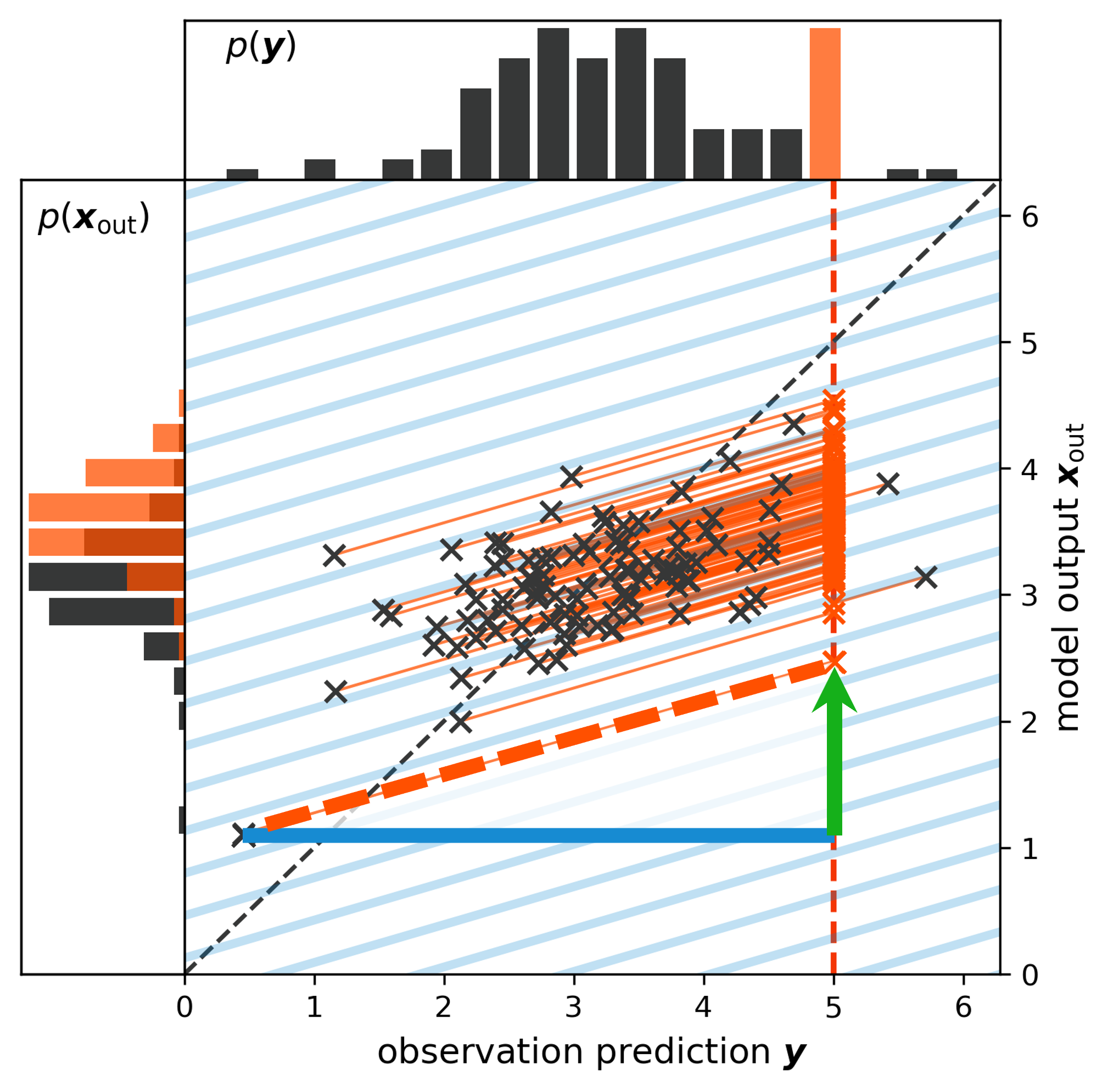
Fig. 65 An illustration of the EnKF’s update procedure.#