Importance sampling

We have encountered the concept of importance sampling earlier in this course, but let us briefly revisit it here again to set us up for its use in particle filters. Consider the following example:

Example: phone survey

We conduct a phone survey about how much time per week people spent working. We want to derive statistics about the population’s workload. It is a common problem in surveys that the demographics of the survey respondents may not reflect the demographics of the general population:

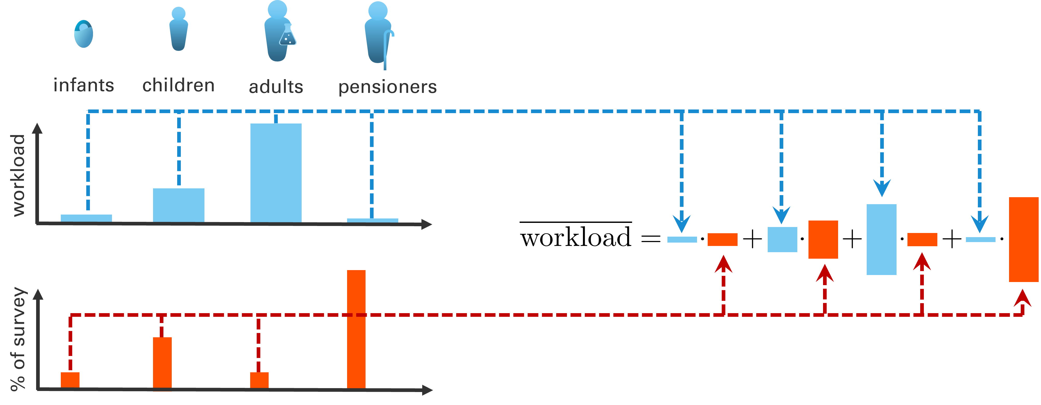
Fig. 70 We want to compute the average workload of the population, but our survey demographics are not representative.

To compensate, we can make use of importance sampling, which introduces an importance weight that “corrects” each response by how much its demographic is over- or underrepresented. As we can see, in this example, it substantially increases the weight of adults, and substantially decreases the weight of pensioners, which were overrepresented in the survey:

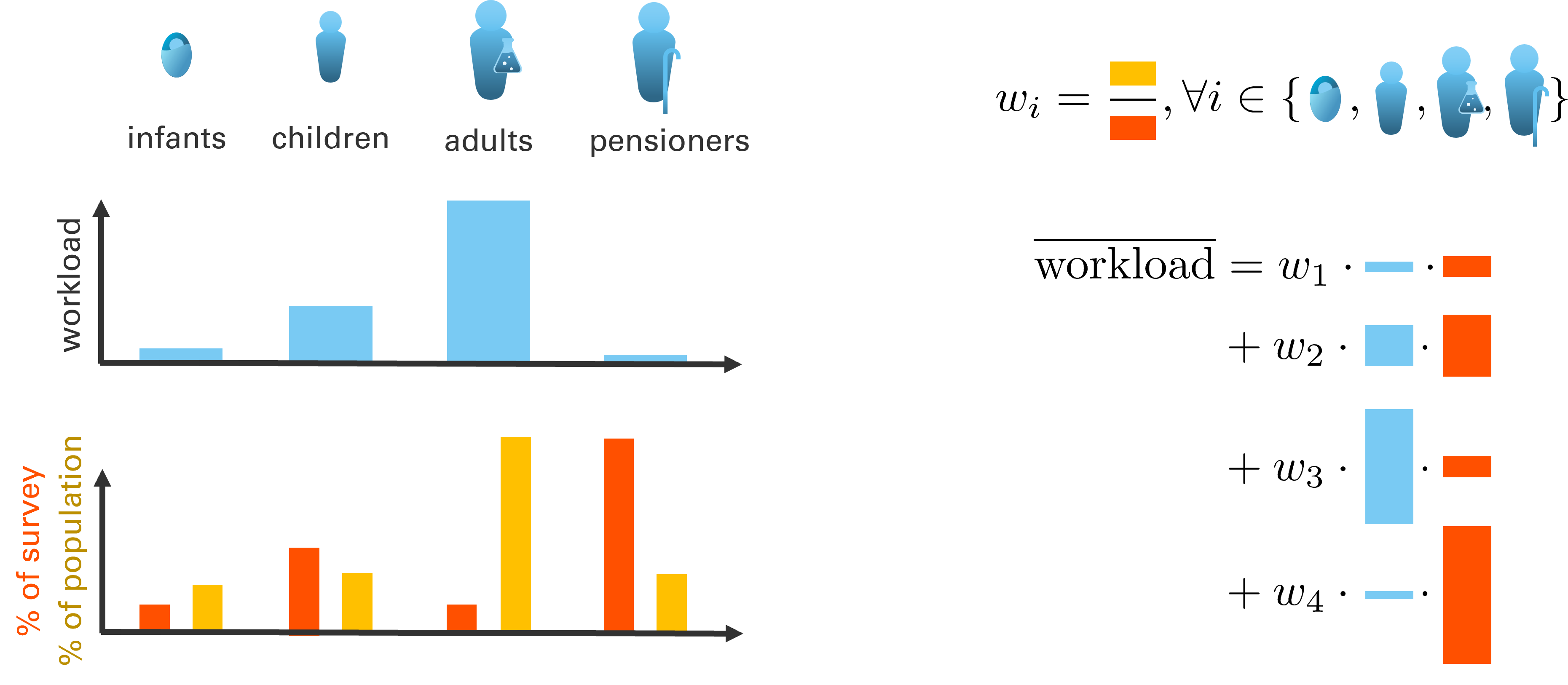
Fig. 71 Assigning importance weights allows us to compensate for this mismatch.

Multiplying the importance weight with the survey fraction of different demographics then lets us compute an aproximate estimate of the mean workload of the general population:

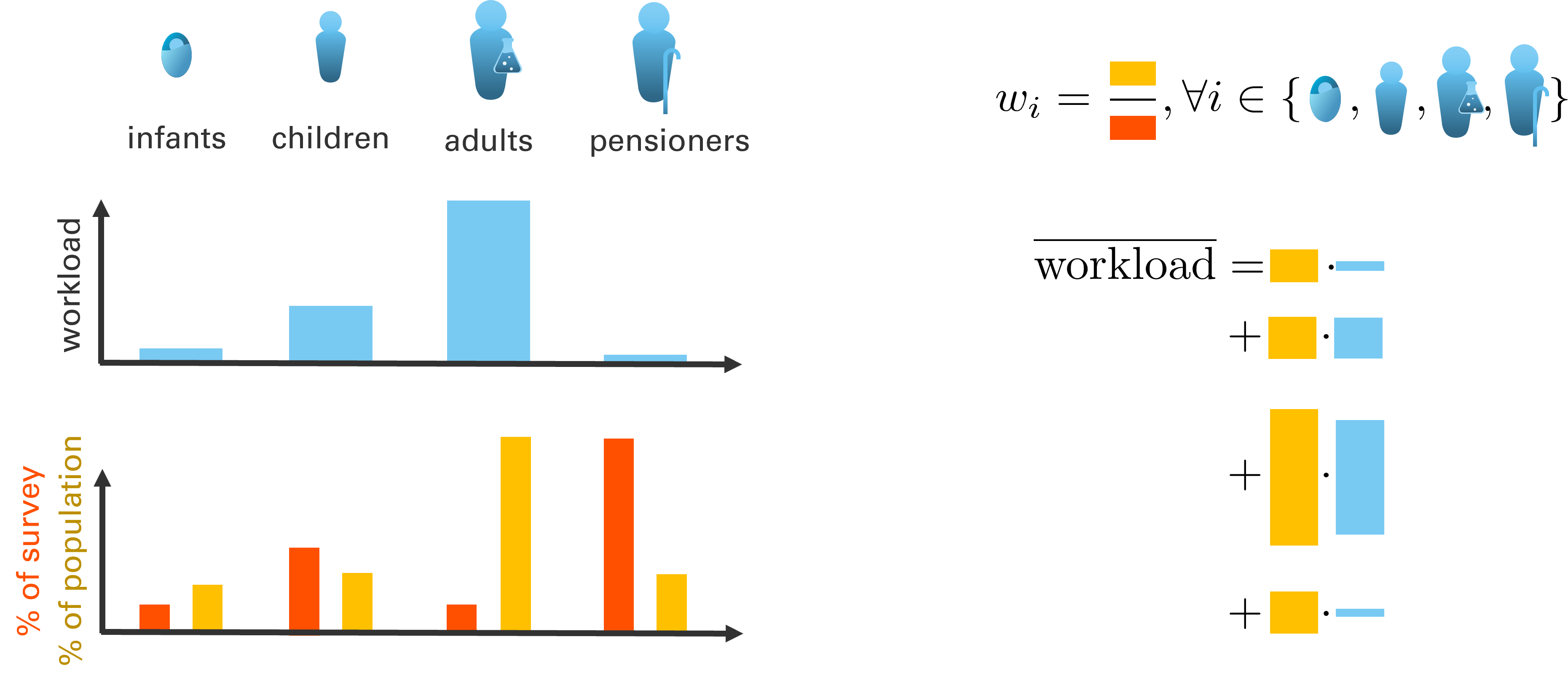
Fig. 72 This allows us to approximately compute the average workload in the population.

In equations

Particle filters rely on ensemble approximations to implement the assimiliation step. In consequence, our target distribution is the filtering posterior \(p(\boldsymbol{x}_{t}|\boldsymbol{y}_{1:t}^{*}) \) and our sampling distribution is the filtering forecast \(p(\boldsymbol{x}_{t}|\boldsymbol{y}_{1:t-1}^{*})\). The update is then applied in several steps:

1. apply importance sampling

   \[p(\boldsymbol{x}_{t}|\boldsymbol{y}_{1:t}^{*}) = p(\boldsymbol{x}_{t}|\boldsymbol{y}_{1:t-1}^{*}) \frac{p(\boldsymbol{x}_{t}|\boldsymbol{y}_{1:t}^{*})}{p(\boldsymbol{x}_{t}|\boldsymbol{y}_{1:t-1}^{*})}\]

2. apply the Monte Carlo approximation (for i.i.d. samples, we have \(w_{t-1}^{n} = 1/N\))

   \[p(\boldsymbol{x}_{t}|\boldsymbol{y}_{1:t}^{*}) \approx \sum_{n=1}^{N} w_{t-1}^{n} \delta(\boldsymbol{X}_{t}^{n}) \frac{p(\boldsymbol{X}_{t}^{n}|\boldsymbol{y}_{1:t-1}^{*})p(\boldsymbol{y}_{t}^{*}|\boldsymbol{X}_{t}^{n})}{p(\boldsymbol{X}_{t}^{n}|\boldsymbol{y}_{1:t-1}^{*})p(\boldsymbol{y}_{t}^{*}|\boldsymbol{y}_{1:t-1}^{*})}\]

3. use Bayes’ Theorem

   \[$p(\boldsymbol{x}_{t}|\boldsymbol{y}_{1:t}^{*}) \approx \sum_{n=1}^{N} w_{t-1}^{n} \delta(\boldsymbol{X}_{t}^{n}) \frac{\cancel{p(\boldsymbol{X}_{t}^{n}|\boldsymbol{y}_{1:t-1}^{*})}p(\boldsymbol{y}_{t}^{*}|\boldsymbol{X}_{t}^{n})}{\cancel{p(\boldsymbol{X}_{t}^{n}|\boldsymbol{y}_{1:t-1}^{*})}p(\boldsymbol{y}_{t}^{*}|\boldsymbol{y}_{1:t-1}^{*})}\]

4. compute the new weights

   \[p(\boldsymbol{x}_{t}|\boldsymbol{y}_{1:t}^{*}) \approx \sum_{n=1}^{N} \delta(\boldsymbol{X}_{t}^{n}) \underbrace{w_{t-1}^{n} \frac{p(\boldsymbol{y}_{t}^{*}|\boldsymbol{X}_{t}^{n})}{p(\boldsymbol{y}_{t}^{*}|\boldsymbol{y}_{1:t-1}^{*})} }_{\text{new weight }w_{t}^{n}}\]

In consequence, the weight \(w_{t}^{n}\) is computed recursively from the weight \(w_{t-1}^{n}\):

\[ p(\boldsymbol{x}_{t}|\boldsymbol{y}_{1:t}^{*}) \approx \sum_{n=1}^{N} \delta(\boldsymbol{X}_{t}^{n}) \underbrace{w_{t-1}^{n} \frac{p(\boldsymbol{y}_{t}^{*}|\boldsymbol{X}_{t}^{n})}{p(\boldsymbol{y}_{t}^{*}|\boldsymbol{y}_{1:t-1}^{*})} }_{\text{new weight }w_{t}^{n}} \rightarrow w_{t}^{n} = w_{t-1}^{n} \frac{p(\boldsymbol{y}_{t}^{*}|\boldsymbol{X}_{t}^{n})}{p(\boldsymbol{y}_{t}^{*}|\boldsymbol{y}_{1:t-1}^{*})} \]

In practice, we do not know the normalizing factor \(p(\boldsymbol{y}_{t}^{*}|\boldsymbol{y}_{1:t-1}^{*})\). Particle filters instead normalize the sample weights within the ensemble:

1. compute the unnormalized weights

   \[\widehat{w}_{t}^{n} = w_{t-1}^{n} p(\boldsymbol{y}_{t}^{*}|\boldsymbol{X}_{t}^{n}) \]

2. normalize weights over ensemble

   \[w_{t}^{n} = \frac{\widehat{w}_{t}^{n}}{\sum_{i=1}^{N}\widehat{w}_{t}^{i}}\]

Example: painting with importance sampling

This process may be a bit abstract, so the interactive element below highlights some of the principles behind importance sampling. Experiment with the element and try to develop intuition for when importance sampling works well, and when it doesn’t.

Fig. 73 Select a 2D distribution to sample, and then select another distribution you want to approximate with importance sampling. Sample weight is represented with opacity: high weights are opaque, low weights are close to transparent. Why combinations of distributions work well, which don’t, and why?