Multivariate Data Exploration

We have already seen the steps required to explore observations of a phenomenon of interest. These steps provid an overall understanding of whether trends or patterns are present and how to derive its statistical characteristics by fitting a probability distribution to the observed data.

However, many phenomena cannot be fully understood by examining observations in isolation. To gain a more complete understanding, we must investigate observations of each component of the phenomenon and the possible interactions among them.

Examples of phenomena include:

• Compound coastal flooding, where storm surge, rainfall, and river discharge interact to produce extreme sea water levels.

• Loads on offshore structures, where wind, wave height, and current velocity jointly influence structural response.

• Climate change and health impacts, where temperature, air pollution, and humidity collectively affect human well-being.

This leads us to the need for multivariate data exploration, where we can capture dependencies, interactions, and more complex structures within the data. Following this exploratory phase, a multivariate statistical model can be developed to formally describe these relationships.

In the following sections, we focus on the bivariate case, where we investigate the interaction between two dependent variables, denoted by \(X\) and \(Y\), and construct statistical models to describe their joint behavior.

Selecting Events of interest

In engineering applications, where design or risk assessment procedures are often of interest, characterizing the joint occurrence of two variables is of great importance. For instance, when designing coastal structures, the combination of water level and wave height can impose much greater stress on the structure than when either acts alone.

In such cases, it is essential that the observations used for analysis are representative of the actual loading conditions experienced by the structure. In other words, data on both variables should be collected in a way that reflects their joint impact. This consideration is particularly relevant when analyzing extreme events.

While we could select maxima for each variable independently, their occurrences in time might not represent the physical reality of joint loading conditions. To better capture these conditions, observations can be selected following the concomitant approach. This approach involves identifying extreme values for one variable and then selecting the corresponding observations of the other variable. These may not occur at the exact same time but within a reference time window during which their combined effect on the system is physically meaningful. In this sense, the concomitant event represents an extreme in impact, even though the underlying physical drivers do not necessarily reach their individual maxima simultaneously.

Similarly, the selection can start from a realized impact, for example, a flood event, and the underlying physical drivers that, within a representative time window, led to that event can then be identified.

Measuring Dependence via Correlation

Assuming that the data selection procedure has produced two time series, \(X\) and \(Y\), we can quantify their dependence using correlation coefficients. Correlation coefficients provide a measure of the strength and direction of the relationship between two variables. The three most commonly used correlation coefficients — Pearson, Spearman, and Kendall — all range between -1 and 1, but their interpretations differ.

• Pearson correlation coefficient (linear correlation):

  \[ \rho_{X,Y} = \frac{\operatorname{cov}(X, Y)}{\sigma_X \, \sigma_Y} \]

  where \(\operatorname{cov}(X, Y)\) is the covariance between \(X\) and \(Y\), and \(\sigma_X\) and \(\sigma_Y\) are their standard deviations. Pearson’s coefficient captures linear dependence between the variables. A value of +1 indicates a perfect linear positive relationship, -1 indicates a perfect linear negative relationship, and 0 indicates no linear association (though the variables may still be dependent in a nonlinear way).

• Spearman’s rank correlation coefficient (monotonic dependence based on ranks):

  \[ \rho_{S} = \frac{\operatorname{cov}(R_X, R_Y)}{\sigma_{R_X} \, \sigma_{R_Y}} \]

  where \(R_X\) and \(R_Y\) are the ranks of \(X\) and \(Y\), respectively. Spearman’s \(\rho_S\) measures monotonic relationships, regardless of whether they are linear. A value of +1 indicates a perfect monotonic increasing relationship, -1 a perfect monotonic decreasing relationship, and 0 indicates no monotonic association. Spearman is robust to outliers and can capture nonlinear but monotonic dependence.

• Kendall’s tau coefficient (rank concordance measure):

  \[ \tau = \frac{2}{n (n - 1)} \sum_{i < j} \operatorname{sign}(x_i - x_j) \, \operatorname{sign}(y_i - y_j) \]

  where \(\operatorname{sign}(\cdot)\) returns \(+1\) if its argument is positive, \(-1\) if negative, and \(0\) if the arguments are equal. A value of \(+1\) indicates perfect concordance (all pairs of observations agree in order), \(-1\) indicates perfect discordance (all pairs disagree in order), and \(0\) indicates no association. Kendall’s tau is nonparametric and robust to nonlinearities, focusing on the probability that pairs of observations are concordant or discordant.

In summary, while all three coefficients are bounded between -1 and 1, Pearson captures linear dependence, Spearman captures monotonic relationships, and Kendall quantifies pairwise concordance.

Visualizing Dependence and Data Transformation

The correlation coefficients introduced earlier provide an overall measure of the dependence between two variables. To investigate these relationships more deeply and to explore how the data relate to each other, visualization plays a key role.

For univariate data, classical tools such as histograms are generally sufficient to examine the shape and variability of individual variables. However, in the case of dependent data, indicidual plots cannot capture the interactions between variables. A common first step is to create pairwise plots of the variables, or scatter plots. In these plots, what happens with each variable on its own is combined with how the variables interact, which can make it hard to see their actual dependence structure

To better isolate the contribution of the dependence structure, it is often useful to transform the data, allowing the joint relationships to be visualized independently of the individual distributions. This provides a clearer view of the underlying dependence between the variables.

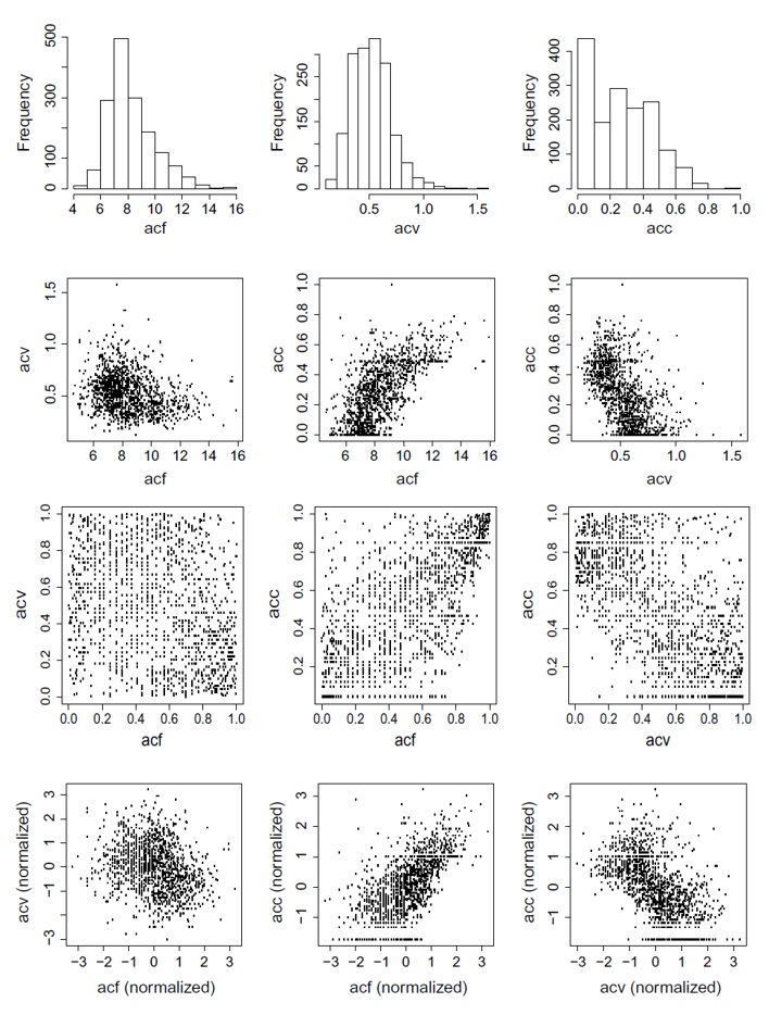
Fig. 28 Data of chemical components of wine: acf = fixed acidity, acv = volatile acidity, acc = citric acid. Row 1: individual histograms. Row 2: scatter plots of pairs of chemicals acf versus acv (left), acf versus acc (middle), acv versus acc (right). Row 3: Scatter plots of the same pairs after transforming the data using the Probability Integral Transform. Row 4: scatter plots of pairs after transforming the data into standard normal variables (normalized). Modified figure 1.4 and 1.5 from Czado C. (2019)

From the figure above, we can see that histograms provide an understanding of the variability of each variable but do not provide information on their relative behaviour (row 1). Scatter plots can help. However, the scale of each variable can influence our understanding of the dependence. For example, from the scatter plots in row 2, \(acf\) has a range of variability from 4 to 16, which is ten times larger than the other two variables (\(acc\) from 0 to 1 and \(acv\) from 0 to 1.5). We see a positive relationship between \(acf\) and \(acc\) (both increase together) and a negative relationship between \(acf\) and \(acv\), and between \(acv\) and \(acc\) (one increases while the other decreases, and vice versa).

We get more information in row 3 (which is also the copula space, as we will see later). We see that \(acf\) and \(acv\) (left) have very little association (dots scattered randomly); \(acf\) and \(acc\) (middle) show clear association in the upper-right corner, meaning that high values are more strongly associated than lower values; \(acv\) and \(acc\) (right) show negative dependence. In row 4, the scatter plots with normalized data further highlight the dependence structure of the data.

The scatterplots in rows 3 and 4 were produced using transformed versions of the data to better highlight their dependence structure. We now formalize these transformations, which form the basis for modelling dependence with copula functions, as we see in the next sections. To do so, we define the following scales:

Original Scale. Two random variables \(X\) and \(Y\) with probability density functions (pdf) \(f_X(x)\) and \(f_Y(y)\) and cumulative distribution functions (cdf) \(F_X(x)\) and \(F_Y(y)\). They can take any observed values in their own units, e.g., precipitation and discharge; traffic load and stress.

Copula Scale. The two variables are transformed via their cdfs (either empirical or theoretical), such that \(u_1 = F_X(x)\) and \(u_2 = F_Y(y)\). Following the probability integral transform, \(u_1\) and \(u_2\) are uniformly distributed between 0 and 1.

Normalized Scale. The two variables are transformed again via \(\Phi\), the standard normal distribution. Hence, \(z_1 = \Phi^{-1}(u_1) = \Phi^{-1}(F_X(x))\) and \(z_2 = \Phi^{-1}(u_2) = \Phi^{-1}(F_Y(y))\). \(\Phi\) is the cdf of a standard normal distribution.