The integrated approach

The integrated approach#

In the integrated approach, we treat the time series $X_t$, including its deterministic component, as stochastic and fit a statistical distribution to it with time-dependent parameters. This approach implies that the distributions modeling $X_t$ belong to the same family, but the parameters vary in accordance with the deterministic component $D(t)$ identified during the exploratory phase. Such a construction can be generalized to capture not only temporal changes but also variations associated with a related physical covariate, for example, changes in temperature corresponding to atmospheric $CO_2$ levels.

This approach can be applied to any distribution. However, here we focus on its application to extreme value analysis because of the long tradition of the statistical theory of extreme values in engineering design, e.g., in estimating “the 100-year event”.

Block Maxima and the Generalized Extreme Value Distribution#

The block maxima method is a common approach in extreme value theory to select extreme events, where a time series is divided into blocks (e.g., yearly or monthly), and only the maximum value from each block is selected. It is possible to show that, the vector of maximum values per block converge to a distribution of the Generalized Extreme Value (GEV) family of distributions, which is given by

\[ G(x) = \exp\left\{ -\left[ 1 + \xi \left( \frac{x - \mu}{\sigma} \right) \right]^{-1/\xi} \right\}, \]

for $ 1 + $\xi$ (x - $\mu$)/$\sigma$ > 0 $, where $\mu$ is the location parameter (or the center of the distribution), $\sigma$ > 0 is the scale parameter (the size of the deviations about the location parameter), and $\xi$ is the shape parameter (or the tail decays).

Depending on the behaviour of the tail of the distribution, which is governed by the shape parameter $\xi$, the GEV distribution takes on different forms. Specifically, it includes three distinct families as special cases: the Gumbel ($\xi = 0$), Fréchet ($\xi > 0$), and Reverse Weibull ($\xi < 0$). More specifically, $\xi$ determines how the distribution accommodates the extreme values among the already extreme observations. When $\xi > 0$, the distribution exhibits a heavy tail, as in the Fréchet case, allowing for the possibility of very large extreme values. Conversely, when $\xi < 0$, corresponding to the Reverse Weibull case, the distribution has a finite upper bound, implying that extremes are bounded. The intermediate case, $\xi = 0$, corresponds to the Gumbel distribution, which is light-tailed.

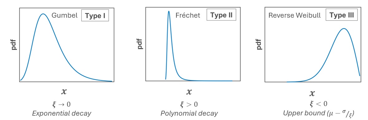
../_images/xi_changes.jpg — Fig. 22 The GEV distribution for different tail behaviour (different $\xi$) .#

In general, changes in the parameters of the GEV distribution reflect the changes observed in the time series. Changes in the average behaviour of the extreme lead to changes in the location parameter, i.e., higher average behaviour corresponds to higher $\mu$. Changes in the variability of the observations lead to changes in $\sigma$. However, it is worth noticing that $\mu$ and $\sigma$ do not correspond to the sample meand and sample standard deviation.

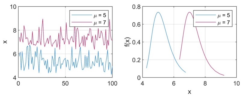
../_images/mu_changes.jpg — Fig. 23 Effect of changes in the location parameter $\mu$.#

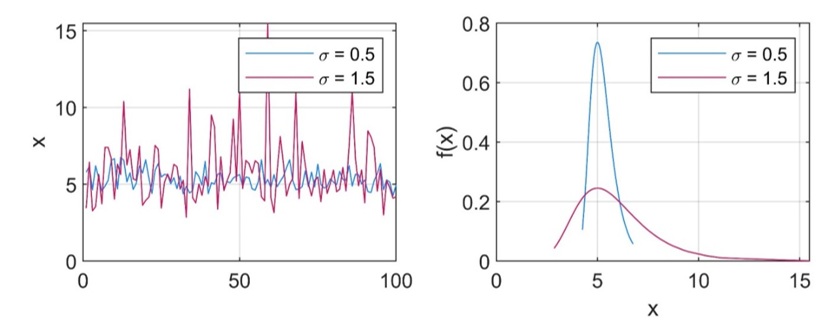
../_images/si_changes.jpg — Fig. 24 Effect of changes in the scale parameter $\sigma.#

GEV under the nonstationary assumption.#

We now examine how the GEV distribution can gradually shift by introducing time as a covariate. In other words, one or more parameters of the GEV are expressed as functions of time, i.e., $\mu(t)$, $\sigma(t)$, and $\xi(t)$.

One possible way to express this model is:

\[ \mu(t) = \mu_0 + \mu_1 t, \quad \ln (\sigma(t)) = \sigma_0 + \sigma_1 t, \quad \xi(t) = \xi. \]

In this example, both the location and the (log-transformed) scale parameters change linearly with time, while the shape parameter is assumed to remain constant. The log transformation ensures that $\sigma(t) > 0 $, since a scale value must always be positive. Moreover, this model implies that at any specific point in time, the distribution of the maximum still follows a standard GEV distribution. The parameter $\mu_1$, the slope of the linear trend in $\mu(t)$, tells us how the center of the distribution changes over time. Similarly, $\sigma_1$ represents how much the variability of the extremes changes each year (or season).

It is possible to extend this framework to other types of functions, such as quadratic or sinusoidal forms. It is also possible to replace the time-dependent variability with variability explained by a physically based covariate, i.e., $\mu(x_c)$, $\sigma(x_c)$, and $\xi(x_c)$.

This framework can be further generalized using Generalized Additive Models for Location, Scale, and Shape (GAMLSS). GAMLSS is a flexible statistical framework that allows the parameters of a chosen parametric distribution to vary as functions of explanatory variables. In GAMLSS, each of these parameters can be modeled as a function of covariates, such as time, using linear terms, smooth functions (e.g., splines), or even random effects:

\[\begin{split} \begin{aligned} g_1(\mu) &= \eta_1 = f_1(t), \\ g_2(\sigma) &= \eta_2 = f_2(t), \\ g_3(\xi) &= \eta_3 = f_3(t), \end{aligned} \end{split}\]

where $g_i(\cdot)$ are appropriate link functions and $f_i(t)$ are smooth functions of time.

This means that the simple linear trend model can be seen as a special case of GAMLSS, where only the location parameter is modeled linearly and the other parameters are held constant. By using GAMLSS, we can not only capture trends in the mean, but also detect changes in variability, asymmetry, and tail behavior over time. This provides a much richer and more realistic description of the distribution of extremes. At the same time, care should be given to aviod overfitting.

Fitting a nonstationary distribution#

Under the assumption of nonstationarity, the distribution includes at least one additional parameter compared to its stationary counterpart. For instance, if a linear trend is introduced in the location parameter, it is described by two parameters: the slope and the intercept. Hence, the GEV has 4 paramerts: $\mu_1$, $\mu_0$, $\sigma$, and $\xi$.

The Maximum Likelihood Estimation (MLE) method can be used to fit a distribution to the data. In MLE, given a set of observations $x_{\text{obs}}$, the estimated parameter set $\theta = \{\mu_0, \mu_1, \dots\}$ is the one that maximizes the likelihood function.

Another approach to estimate $\theta$ given $x_{\text{obs}}$ is by applying Bayes’ Theorem. In this approach, $\theta$ is treated as a random variable. More specifically, we obtain $\theta$ from the following posterior distribution:

\[ p(\theta|x_{\text{obs}}) = p(\theta)p(x_{\text{obs}}|\theta) \]

where $p(\theta)$ is called prior and $p(x_{\text{obs}}|\theta)$ is the likelihood. Specifically for the GEV distribution with a linear trend in the location parameter $\mu(t) = \mu_0 + \mu_1t$, we have:

\[ p(\mu_0,\mu_1,\sigma,\xi | x_{\text{obs}}) = p(\mu_0)p(\mu_1)p(\sigma)p(\xi)\prod_{i=1}^N p(x_i|\mu_0,\mu_1,\sigma,\xi | x_{\text{obs}}) \]

assuming that the parameters and the observations are independent.

Diagnostincs.#

After estimating and selecting among possible models, it is essential to verify that the final model adequately represents the data. In the non-stationary case, however, the lack of homogeneity in the distributional assumptions across observations requires modifications to standard model-checking procedures. Diagnostic tests such as probability and quantile plots, which are both graphical tools where the theoretical and the empirical probability/quantile is compared against each other, can still be implemented. However, this requires a transformation of the random variable (observations) considered.

Given a set of observations $Z$ and parameters of a GEV distribution fitted to the data $\mu(t)$, $\sigma(t)$, and $\xi(t)$, the transformed variable $\tilde{Z}$ is

\[ \tilde{Z} = \frac{a}{\xi(t)}log(1 + \xi(t)(\frac{Z(t) - \mu(t)}{\sigma(t)})) \]

It is possible to prove that $\tilde{Z}$ follow a standard stationary Gumber distribution, allowing comparison between empirical and theoretical model.