Data Exploration#
Before conducting a detailed nonstationary analysis, it is useful to begin with a general exploration of the data to better understand its key characteristics and potential sources of variability.
A time series is a sequence of quantitative observations recorded over time, typically at regular intervals. It can be expressed as \(X_t = \{x_1, x_2, \dots, x_N\}\), where \(x_i\) denotes the value observed at time \(i\). From a stochastic perspective, a time series can be viewed as a realization of an underlying random process \(\{X_t\}\) with \(x_i\) representing the observation at time \(i\). A time series, or a collection of such observations, is often referred to as data.
A stochastic process \(\{X_t\}\) is said to be strictly stationary if for every integer \(k\) and for all time indices \(t_1, t_2, \dots, t_k\), the joint distribution of \((X_{t_1}, X_{t_2}, \dots, X_{t_k})\) is identical to that of \((X_{t_1+h}, X_{t_2+\tau}, \dots, X_{t_k+h})\) for any time shift \(h\).
A weak stationary process refers to a process in which only the mean and covariance are functions of the lag \(h\).
These observations often reflect an underlying physical process that shapes the structure and dynamics of the series. Hence, we look for a mathematical model that plausibly describes the observations.
The first step is to visually examine the data in the context of existing knowledge about the processes that generate it. It is conventional to display a time series graphically by plotting the values of the random variables on the y-axis with the time scale as the x-axis. It is often helpful to join the points from one time period to the next to get a sense of the continuous pattern behind the data, like a seasonal cycle or a linear trend.
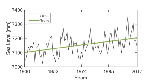
Fig. 20 Mean sea level and detected trend.#
If prior knowledge exists about the variability of the observations as a function of another variable, e.g., temperature and \(CO_2\) in the atmosphere, the two observations can be plotted alongside each other.
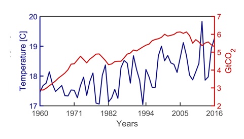
Fig. 21 Mean Global Temperature in response to emissions.#
Testing for trend: The Mann-Kenadall Trend Test A visual inspection provide a first insight into whether trends or patterns exist in the observations collected. However, it is also useful to carry out statistical tests, i.e., test of hypothesis, to evaluate the significance of such trend and patterns observed. Test of hypotesis can be conducted to tests changes in mean values, e.g., such as the Student’s t-test, or step changes in the average level of the time series, e.g., Pettitt’s test. Similarly, tests can be conducted to detect changes in the variance, e.g., White’s tests for heteroschedasticity.
To test whether there is a monotonic trend in the time series, e.g., the observations constatly increase/decrease over time, we can implement the Mann-Kendall (MK) trend test. The MK test is non-parametric, meaning that it does not assume normality or linearity, making it especially useful for environmental data. The hypotheses are:
Null hypothesis \(H_0\): There is no monotonic trend (data are independent).
Alternative hypothesis \(H_1\): There is a monotonic trend (either increasing or decreasing).
Given a time series \(X = x_1, x_2, \dots, x_n \) of length \(N\), the statistic \(S\) of the test is computed by comparing each observation in a time step with the observations at later time. More specifically:
\( S = \sum_{i=1}^{n-1} \sum_{j=i+1}^{n} \operatorname{sgn}(x_j - x_i) \)
where
\( \operatorname{sgn}(x_j - x_i) = \begin{cases} +1 & \text{if } x_j - x_i > 0 \\ 0 & \text{if } x_j - x_i = 0 \\ -1 & \text{if } x_j - x_i < 0 \end{cases} \)
and variance (assuming that all the observations are unique, i.e., no ties)
\( Var(S) = \frac{n(n-1)(2n+5)}{18} \)
In essence, \(S\) counts the number of times the series moves upward versus downward, providing a measure of the overall direction and consistency of a trend.
To carry out the test of significance, the statistic \(S\) is standardized as
\( Z = \begin{cases} \dfrac{S - 1}{\sqrt{Var(S)}} & \text{if } S > 0 \\ 0 & \text{if } S = 0 \\ \dfrac{S + 1}{\sqrt{Var(S)}} & \text{if } S < 0 \end{cases} \)
where ( Z ) follows approximately a standard normal distribution \(N(0,1)\).
Assuming that the level of significance of the test \(\alpha\) is \(0.05\), the outcome of the test is the following:
If \( |Z| > 1.96 \): Reject \(H_0\) there are enough evidence to reject \(H_0\) so a statistically significant trend exists.
If \( |Z| \leq 1.96 \): Fail to reject \(H_1\), there are no evidence to reject \(H_0\) so no statistically significant trend exists.
Here, \(1.96\) corresponds to the \(97.5^{th}\) percentile of the standard normal distribution, meaning that the probability of observing a value greater than this under the null hypothesis (\(H_0\)) is less than a \(0.05\). In other words, it represents the probability of making an error (Type I ) that we are willing to accept. Note that the level of significance is arbitrary and can be chosen depending on the context.
Instead of choosing a fixed level of significance, we can evaluate the p-value, which represents the probability of observing the test statistic, in this case \(Z\), under the null hypothesis. A small p-value indicates strong evidence against \(H_0\), while a large p-value suggests that the observations are consistent with it.
After identifying a trend, a first-order polynomial (linear) fit, often obtained through linear regression, can provide a simple deterministic approximation of the underlying trend.
It is important to note that the MK trend test fails to detect cyclic patterns, such as seasonal variations, because it is a test for monotonic trend.