Ensemble filters

In the previous lecture, we have discussed the Kalman Filter, which allows us to do closed-form Bayesian filtering if all probability distributions involved are Gaussian, and all models involved are linear. Unfortunately, in real systems, these two assumptions are almost never met: uncertainties often display non-Gaussian features, and interesting dynamics are virtually always nonlinear (in the famous words of Stanisław Ulam: “Using a term like nonlinear science is like referring to the bulk of zoology as the study of non-elephant animals.”).

What can we do in these cases? A practical answer can be found in so-called ensemble filtering algorithms. Instead of attempting inference of closed-form PDFs, ensemble filters instead use a Monte Carlo approach to approximate the underlying distributions of interest. In this course, we will consider two such algorithms:

• the ensemble Kalman filter (EnKF), which is an ensemble variant of the KF that supports nonlinear forecast models and observations model, and

• the particle filter (PF), which is an ensemble filter that uses ideas related to biological evolution, and which is significantly more statistically powerful at the expense of being more sample-inefficient.

The Monte Carlo approximation

Let us begin by recalling the fundamental idea of a Monte Carlo approximation. If we have access to a closed-form PDF \(p(\boldsymbol{x})\), we can do a lot of interesting statistical operations: we can draw samples \(X \sim p(\boldsymbol{x})\) from the PDF, evaluate different expectations, analyze rare events, and so forth. Unfortunately, we rarely have such closed-form PDFs. The key idea behind the Monte Carlo approximation is that if we have access to sufficiently many samples \(X \sim p(\boldsymbol{x})\) but not their generating PDF \(p(\boldsymbol{x})\), we can still do many of these same operations approximately.

For instance, assume you are organizing a board game evening with a large group of friends, but you only brought a single die. Sharing it would be cumbersome, but fortunately, there is an alternative strategy. You could simply roll the die \(1000\) times, write the results on pieces of paper, and put these papers in an urn. Once you have done this, you could replicate a lot of operations with your Monte Carlo samples (the pieces of paper in the urn) that you could also do with the real thing (the die): you can simulate die rolls by simply drawing a paper at random from the urn, or you could analyze the fairness of the die by analyzing the relative frequency of numbers in the urn.

Fig. 62 You plan a relaxing board game evening, but - oh no! - you only brought a single die. No worries. A quick session of rolling that die a thousand times, writing down the results on pieces of paper, and putting these pieces into an urn (Monte Carlo sampling) creates an effective duplicate of the die (the underlying distribution). And it will only be marginally slower than setting up that one complex strategy game your friend always brings along.

Of course, in science and engineering, or setups are a bit more complex than simple die rolls. In the problems we care about, we usually have complex physical models that relate complex input variables to complex output variables. This would then require probability density functions which not only capture the complex relationships encoded in our models, but assign the correct probability density to any conceivable combination of inputs and outputs. This is a near-impossible task.

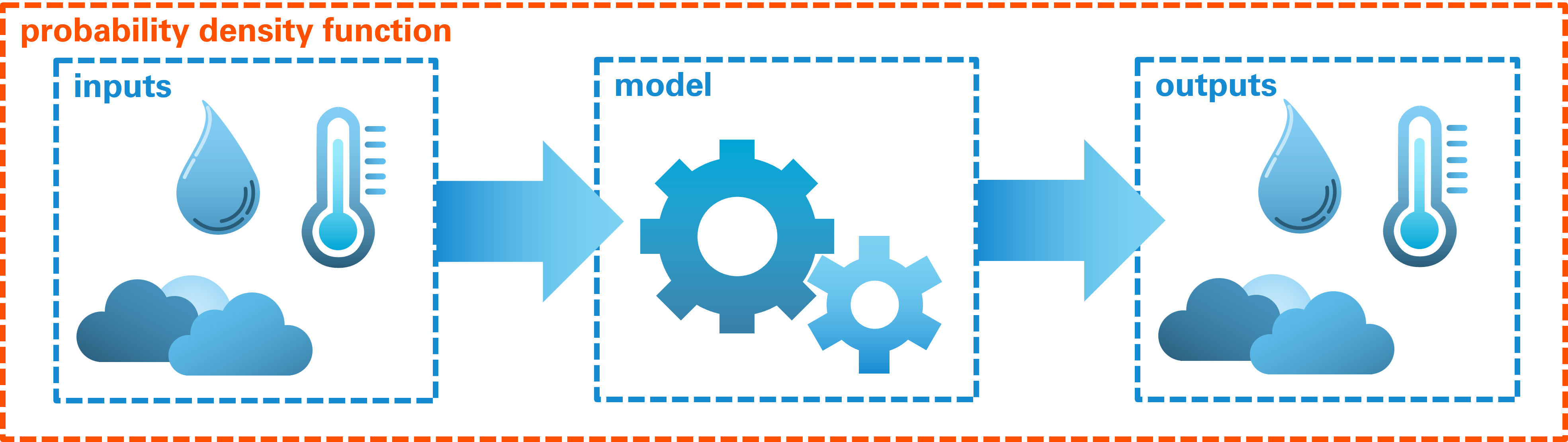
Fig. 63 In many settings, a joint PDF between model inputs and outputs does not only have to capture the physics encoded in the model, but the probability of the inputs and outputs.

A Monte Carlo approximations simplifies this dramatically by considering samples from this unknowable PDF instead. Rather than attempting to describe the relationship for all conceivable combinations of inputs and outputs at once, we can consider an ensemble of input values, run the model for each of them, and obtain the corresponding output values. The resulting joint ensemble then describes some of the relationship between input and output variables.

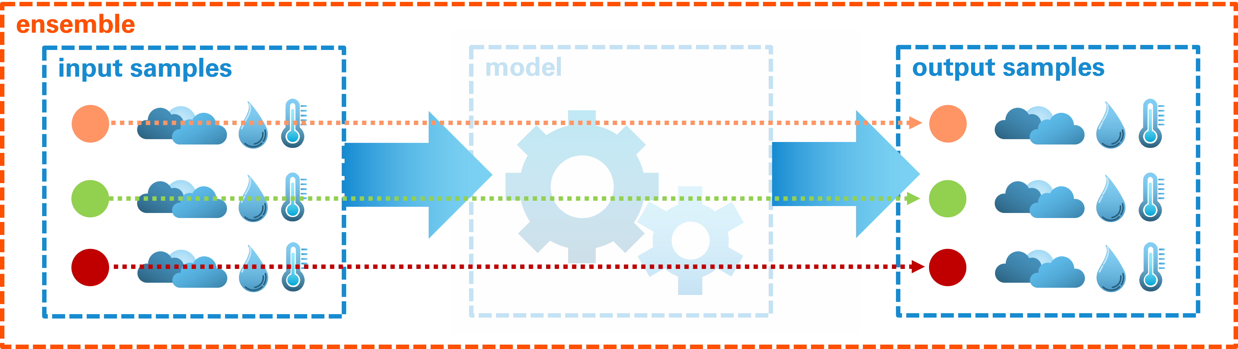
Fig. 64 An ensemble approximation uses the numerical model to establish a relationship between model inputs and model outputs. In the resulting Monte Carlo approximation, the model is only represented indirectly.