2. Modules, conditions, data structures and loops

2. Modules, conditions, data structures and loops#

2.1 Python Modules#

Previously, you have learned how to:

1) initialize variables in Python;
2) perform simple actions with them (eg.: adding numbers together, displaying variables content, etc);
3) work with functions (have your own code in a function to reuse it many times or use a function, which was written by another person).

However, the scope of the last Notebook was limited by your Python knowledge and available functions in standard/vanilla Python (so-called ’built-in’ Python functions). There are not many Python built-in functions that can be useful for you, such as functions for math, plotting, signal processing, etc. Luckily, there are countless modules/packages written by other people.

Python built-in modules#

By installing any version of Python, you also automatically install its built-in modules.

One may wonder — why do they provide some functions within built-in modules, but not directly as a built-in function, such as the abs() or print()?

The answers may vary, but, generally, it is to keep your code clean; compact; and, working.

It keeps your code clean and compact as you only load functions that you need. It keeps your code working as it allows you to define your own functions with (almost) any kind of name, and use them easily, without worrying that you might ’break’ something if there is a function with the same name that does something completely different.

math#

The math module is one of the most popular modules since it contains all implementations of basic math functions (\(sin\), \(cos\), \(exp\), rounding, and other functions — the full list can be found here).

In order to access it, you just have to import it into your code with an import statement. Then using print() to show that math is actually a built-in Python module.

import math
print(math) 

<module 'math' (built-in)>

You can now use its functions like this:

print(f'Square root of 16 is equal to {int(math.sqrt(16))}')

Square root of 16 is equal to 4

You can also use the constants defined within the module, such as math.pi:

print(f'π is equal to {math.pi}')
print('π is equal to {:.2f}'.format(math.pi)) 
print('π is equal to {:.1f}'.format(math.pi))
print('π with two decimals is {:.2f},'
      'with three decimals is {:.3f} and with four decimals is {:.4f}'.\
      format(math.pi, math.pi, math.pi))

π is equal to 3.141592653589793
π is equal to 3.14
π is equal to 3.1
π with two decimals is 3.14,with three decimals is 3.142 and with four decimals is 3.1416

Let’s break it down

print('π is equal to {:.2f}'.format(math.pi)) print the variable up to some decimal, (two for example).
print('π is equal to {:.1f}'.format(math.pi)) change the number 2 on the ‘:.2f’ to print with more (or fewer) decimals.
The last line show how to print is quickly if you have to print a sentence with many variables in it.

More information on printing best practices here.

`math.pi`#

As you can see, both constants and functions of a module are accessed by using: the module’s name (in this case math) and a . followed by the name of the constant/function (in this case pi).

We are able to do this since we have loaded all contents of the module by using the import keyword. If we try to use these functions somehow differently — we will get an error:

print('Square root of 16 is equal to')
print(sqrt(16))

Square root of 16 is equal to
4.0

You could, however, directly specify the functionality of the module you want to access. Then, the above cell would work.

This is done by typing: from module_name import necessary_functionality, as shown below:

from math import sqrt

print(f'Square root of 16 is equal to {int(sqrt(16))}.')

Square root of 16 is equal to 4.

from math import pi

print(f'π is equal to {pi}.')

π is equal to 3.141592653589793.

Listing all functions#

Sometimes, when you use a module for the first time, you may have no clue about the functions inside of it. In order to unveil all the potential a module has to offer, you can either access the documentation on the corresponding web resource or you can use some Python code.

You can listing all contents of a module using dir(). To learn something about, let’s say, hypot thingy you can type the module name - dot -function name, for example math.hypot.

import math
print('contents of math:', dir(math))
print('math hypot is a', math.hypot) 

contents of math: ['__doc__', '__loader__', '__name__', '__package__', '__spec__', 'acos', 'acosh', 'asin', 'asinh', 'atan', 'atan2', 'atanh', 'ceil', 'comb', 'copysign', 'cos', 'cosh', 'degrees', 'dist', 'e', 'erf', 'erfc', 'exp', 'expm1', 'fabs', 'factorial', 'floor', 'fmod', 'frexp', 'fsum', 'gamma', 'gcd', 'hypot', 'inf', 'isclose', 'isfinite', 'isinf', 'isnan', 'isqrt', 'ldexp', 'lgamma', 'log', 'log10', 'log1p', 'log2', 'modf', 'nan', 'perm', 'pi', 'pow', 'prod', 'radians', 'remainder', 'sin', 'sinh', 'sqrt', 'tan', 'tanh', 'tau', 'trunc']
math hypot is a <built-in function hypot>

You can also use ? or ?? to read the documentation about it in Python

math.hypot?

Docstring:
hypot(*coordinates) -> value

Multidimensional Euclidean distance from the origin to a point.

Roughly equivalent to:
    sqrt(sum(x**2 for x in coordinates))

For a two dimensional point (x, y), gives the hypotenuse
using the Pythagorean theorem:  sqrt(x*x + y*y).

For example, the hypotenuse of a 3/4/5 right triangle is:

    >>> hypot(3.0, 4.0)
    5.0
Type:      builtin_function_or_method

Python third-party modules#

Besides built-in modules, there are also modules developed by other people and companies, which can be also used in your code.

These modules are not installed by default in Python, they are usually installed by using the ’pip’ or ’conda’ package managers and accessed like any other Python module.

This YouTube video explains how to install Python Packages with ’pip’ and ’conda’.

numpy#

The numpy module is one of the most popular Python modules for numerical applications. Due to its popularity, developers tend to skip using the whole module name and use a smaller version of it (np). A different name to access a module can be done by using the as keyword, as shown below.

import numpy as np
print(np)
x = np.linspace(0, 2 * np.pi, 50)
y = np.cos(x)
print('\n\nx =', x)
print('\n\ny =', y)

<module 'numpy' from 'c:\\ProgramData\\Anaconda3\\lib\\site-packages\\numpy\\__init__.py'>


x = [0.         0.12822827 0.25645654 0.38468481 0.51291309 0.64114136
 0.76936963 0.8975979  1.02582617 1.15405444 1.28228272 1.41051099
 1.53873926 1.66696753 1.7951958  1.92342407 2.05165235 2.17988062
 2.30810889 2.43633716 2.56456543 2.6927937  2.82102197 2.94925025
 3.07747852 3.20570679 3.33393506 3.46216333 3.5903916  3.71861988
 3.84684815 3.97507642 4.10330469 4.23153296 4.35976123 4.48798951
 4.61621778 4.74444605 4.87267432 5.00090259 5.12913086 5.25735913
 5.38558741 5.51381568 5.64204395 5.77027222 5.89850049 6.02672876
 6.15495704 6.28318531]


y = [ 1.          0.99179001  0.96729486  0.92691676  0.8713187   0.80141362
  0.71834935  0.6234898   0.51839257  0.40478334  0.28452759  0.1595999
  0.03205158 -0.09602303 -0.22252093 -0.34536505 -0.46253829 -0.57211666
 -0.67230089 -0.76144596 -0.8380881  -0.90096887 -0.94905575 -0.98155916
 -0.99794539 -0.99794539 -0.98155916 -0.94905575 -0.90096887 -0.8380881
 -0.76144596 -0.67230089 -0.57211666 -0.46253829 -0.34536505 -0.22252093
 -0.09602303  0.03205158  0.1595999   0.28452759  0.40478334  0.51839257
  0.6234898   0.71834935  0.80141362  0.8713187   0.92691676  0.96729486
  0.99179001  1.        ]

Let’s break it down

The code uses the numpy library in Python to perform the following tasks:

It imports the numpy library.
It prints information about the numpy package.
It creates an array x with 50 equally spaced values between \(0\) and \(2\pi\).
It calculates the cosine of each element in the array x and stores the results in the array y.
It prints the arrays x and y.

In summary, the code imports the numpy library, creates an array x with \(50\) evenly spaced elements between \(0\) and \(2\pi\), calculates the cosine of each element in x, and finally prints the arrays x and y.

You will learn more about this and other packages in separate Notebooks since these packages are frequently used by the scientific programming community.

`matplotlib`#

The matplotlib module is used to plot data. It contains a lot of visualization techniques and, for simplicity, it has many submodules within the main module. Thus, in order to access functions, you have to specify the whole path that you want to import.

For example, if the function you need is located within the matplotlib module and pyplot submodule, you need to import matplotlib.pyplot; then, the access command to that function is simply pyplot.your_function().

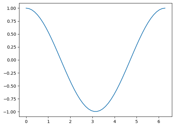
Below we use the data generated in the previous cell to create a simple plot using the pyplot.plot() function:

In order to import a submodule the parent module must also be specified. It is common to import matplotlib.pyplot as plt.

The plt.plot() function takes x-axis values as the first argument and y-axis, or \(f(x)\), values as the second argument

import matplotlib.pyplot as plt
plt.plot(x, y)

[<matplotlib.lines.Line2D at 0x17fff89af70>]

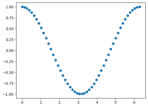
../../_images/7a2bc3eeced6fe24c394dc9650ebe9a71e17468b0c1b9f2f27538b0cacda3adf.png

plt.scatter() works in a similar way, but it does not connect the dots.

plt.scatter(x, y)

<matplotlib.collections.PathCollection at 0x17fff8f4f40>

../../_images/10e5cdb45cdfb5e9acb02bf1d35f3cbc3df9bebdbfd37c4c16ef3e26d516987e.png

Loading Python files as modules#

Finally, you can also load your own (or somebody else’s) Python files as modules. This is quite helpful, as it allows you to keep your code projects well-structured without the need to copy and paste everything.

In order to import another *.py file as a module, you only need to have that file and your Notebook file in the same directory and use the import keyword. More info on this here.

2.2 Conditions and `if` statements#

In previous Sections you have learned how to create variables, alter them with the help of operators and access the code of professional software developers/scientists. With this, you can already do plenty of stuff in Python. However, it still lacks versatility. If you want to apply other processing techniques for other data — you would need to manually rewrite your code and then change it back once the data changes again. Not that handy, right?

In this Section you will learn how to steer the flow of your code — process data differently based on some conditions. For that you will learn a construction called the if statement.

`if` keyword

#

The if statement in Python is similar to how we use it in English. ”If I have apples, I can make an apple pie” — clearly states that an apple pie will exist under the condition of you having apples. Otherwise, no pie.

Well, it is the same in Python:

amount_of_apples = 0

if amount_of_apples > 0:
    print("You have apples!\nLet's make a pie!")

print('End of the cell block...')

End of the cell block...

As you can see - nothing is printed besides ’End of the cell block…’.

But we can clearly see that there is another print statement! Why it is not printed? Because we have no apples… thus no pie for you.

Let’s acquire some fruit and see whether something will change…

Adding 5 apples to our supply:

amount_of_apples += 5

if amount_of_apples > 0:
    print("You have apples!\nLet's make a pie!") 

print('End of the cell block...')

You have apples!
Let's make a pie!
End of the cell block...

Now you can see that the same if statement prints text. It happened because our statement amount_of_apples > 0 is now True.

That’s how an if statement works — you type the if keyword, a statement and a colon. Beneath it, with an indentation of 4 spaces (1 tab), you place any code you want to run in case that if statement is True. This indentation is the same as described in Notebook 1 when defining a function.

If the result of the conditional expression is False, then the code inside of the if statement block will not run. Here’s another example:

my_age = 25

if my_age >= 18 and my_age <= 65:
    print("I'm an adult, I have to work right now :(")

print('End of the cell block...')

I'm an adult, I have to work right now :(
End of the cell block...

Slightly different setting but still the same construction. As you can see in this case, the condition of the if statement is more complicated than the previous one. It combines two smaller conditions by using the keyword and. Only if both conditions are True the final result is True (otherwise it would be False).Thus, the condition can be as long and as complicated as you want it to be, just make sure that it is readable.

`elif` keyword

Now, let's add a bit more logic to our last example:

my_age = 25

if my_age >= 18 and my_age <= 65:
    print("I'm an adult, I have to work right now :(")
elif my_age > 65:
    print("I can finally retire!")

print('End of the cell block...')

I'm an adult, I have to work right now :(
End of the cell block...

Still the same output, but what if we change our age…

my_age = 66

if my_age >= 18 and my_age <= 65:
    print("I'm an adult, I have to work right now :(") # msg #1
elif my_age > 65:
    print("I can finally retire!") # msg #2

print('End of the cell block...')

I can finally retire!
End of the cell block...

See.. we have a different output. Changing the value of our variable my_age changed the output of the if statement. Furthermore, the elif keyword helped us to add more logic to our code. Now, we have three different output scenarios:

print message #\(1\) if my_age is within the \([18, 65]\) range;
print message #\(2\) if my_age is bigger than \(65\); and,
print none of them if my_age doesn’t comply with none of the conditions (as shown below).

my_age = 15

if my_age >= 18 and my_age <= 65:
    print("I'm an adult, I have to work right now :(") # msg #1
elif my_age > 65:
    print("I can finally retire!") # msg #2

print('End of the cell block...')

End of the cell block...

One can also substitute an elif block by a different if block, however it is preferred to use elif instead to ”keep the condition together” and to reduce code size.

Warning

It is important to know that there should be only one if block and any number of elif blocks within it.

A last example below setting my_age = 88 to run the first elif block and setting my_age = 7 to run the second elif block.

my_age = 88

if my_age >= 18 and my_age <= 65:
    print("I'm an adult, I have to work right now :(")
elif my_age > 65:
    print("I can finally retire!")
elif my_age < 10:
    print("I'm really, really young")


my_age = 7

if my_age >= 18 and my_age <= 65:
    print("I'm an adult, I have to work right now :(")
elif my_age > 65:
    print("I can finally retire!")
elif my_age < 10:
    print("I'm really really young")

print('End of the cell block...')

I can finally retire!
I'm really really young
End of the cell block...

`else` keyword#

We can go even further and add an additional scenario to our if statement with the else keyword. It runs the code inside of it only when none of the if and elif conditions are True:

my_age = 13

if my_age >= 18 and my_age <= 65:
    print("I'm an adult, I have to work right now :(")
elif my_age > 65:
    print("I can finally retire!")
elif my_age < 10:
    print("I'm really really young")
else:
    print("I'm just young")

print('End of the cell block...')

I'm just young
End of the cell block...

On the previous example, since my_age is not between \([18,65]\), nor bigger than \(65\), nor smaller than \(10\), the else block is run.

Below, a final example setting my_age = 27 to run the if block, then setting my_age = 71 to run the first elif block. To run the second elif block we set my_age = 9 . Finally, setting my_age = 13 to run the else block.

my_age = 27

if my_age >= 18 and my_age <= 65:
    print("I'm an adult, I have to work right now :(")
elif my_age > 65:
    print("I can finally retire!")
elif my_age < 10:
    print("I'm really really young")
else:
    print("I'm just young")

print('End of the cell block...')
print('------------------------')

my_age = 71

if my_age >= 18 and my_age <= 65:
    print("I'm an adult, I have to work right now :(")
elif my_age > 65: # first elif block
    print("I can finally retire!")
elif my_age < 10:
    print("I'm really really young")
else:
    print("I'm just young")

print('End of the cell block...')
print('------------------------')


my_age = 9

if my_age >= 18 and my_age <= 65:
    print("I'm an adult, I have to work right now :(")
elif my_age > 65:
    print("I can finally retire!")
elif my_age < 10: # second elif block
    print("I'm really really young")
else:
    print("I'm just young")

print('End of the cell block...')
print('------------------------')


my_age = 13

if my_age >= 18 and my_age <= 65:
    print("I'm an adult, I have to work right now :(")
elif my_age > 65:
    print("I can finally retire!")
elif my_age < 10:
    print("I'm really really young")
else: # else block
    print("I'm just young")

print('End of the cell block...')
print('------------------------')

I'm an adult, I have to work right now :(
End of the cell block...
------------------------
I can finally retire!
End of the cell block...
------------------------
I'm really really young
End of the cell block...
------------------------
I'm just young
End of the cell block...
------------------------

That’s almost everything you have to know about if statements! The last two things are:

It goes from top to bottom. When the first condition to be True runs, it skips all conditions after it — as shown below:

random_number = 17

if random_number > 35:
    print('Condition #1')
elif random_number > 25:
    print('Condition #2')
elif random_number > 15:
    print('Condition #3')
elif random_number > 5:
    print('Condition #4')
else:
    print('Condition #5')

Condition #3

You can put almost everything inside each condition block and you can define variables within each block:

my_income = 150
my_degree = 'BSc'

if my_degree == 'BSc':
    x = 5
    if my_income > 300:
        b = 2
        print('I am a rich BSc student')
    else:
        print('I am a poor BSc student')

elif my_degree == 'MSc':

    if my_income > 300:
        print('I am a rich MSc student')
    else:
        print('I am a poor MSc student')

print('x =', x)
print('b =', b)

I am a poor BSc student
x = 5

---------------------------------------------------------------------------
NameError                                 Traceback (most recent call last)
Cell In[22], line 20
     17         print('I am a poor MSc student')
     19 print('x =', x)
---> 20 print('b =', b)

NameError: name 'b' is not defined

As you can see, we can make it as complicated as we want in terms of conditional branching.

Additionally, you can see that only variables within the blocks which run were created, while other variables were not. Thus, we have a NameError that we tried to access a variable (b) that was not defined.

2.3 Data Structures#

In this Section you will tackle a data management problem! In the first module you have learned how to create variables, which is cool. But when you populate a lot of variables, or you want to store & access them within one entity, you need to have a data structure.

There are plenty of them, which differ their use cases and complexity. Today we will tackle some of the standard Python built-in data structures. The most popular of those are: list, dict and tuple.

`list`#

First, the easiest and the most popular data structure in Python: list (which is similar to a typical array you could have seen in a different programming language).

You can create a list in the following ways:

Creating an empty list, option 1
Creating an empty list, option 2 - using the class constructor
Creating a list from existing data - option 1
Creating a list from existing data - option 2

#1
empty_list1 = []
print('Type of my_list1 object', type(empty_list1))
print('Contents of my_list1', empty_list1)
print('--------------------')

#2
empty_list2 = list()
print('Type of my_list2 object', type(empty_list2))
print('Contents of my_list2', empty_list2)
print('--------------------')

#3
my_var1 = 5
my_var2 = "hello"
my_var3 = 37.5

my_list = [my_var1, my_var2, my_var3]
print('Type of my_list3 object', type(my_list))
print('Contents of my_list3', my_list)
print('--------------------')


#4
cool_rock = "sandstone" # remember that a string is a collection of characters

list_with_letters = list(cool_rock)

print('Type of my_list3 object', type(list_with_letters))
print('Contents of list_with_letters', list_with_letters)
print('--------------------')

Type of my_list1 object <class 'list'>
Contents of my_list1 []
--------------------
Type of my_list2 object <class 'list'>
Contents of my_list2 []
--------------------
Type of my_list3 object <class 'list'>
Contents of my_list3 [5, 'hello', 37.5]
--------------------
Type of my_list3 object <class 'list'>
Contents of list_with_letters ['s', 'a', 'n', 'd', 's', 't', 'o', 'n', 'e']
--------------------

As you can see, in all three cases we created a list, only the method how we did it was slightly different:

the first method uses the bracket notation.
the second method uses class constructor approach.

Both methods also apply to the other data structures.

Now, we have a list — what can we do with it?

Well… we can access and modify any element of an existing list. In order to access a list element, square brackets [] are used with the index of the element we want to access inside. Sounds easy, but keep in mind that Python has a zero-based indexing (as mentioned in Section 1.4 in Notebook 1).

Note

A zero-based indexing means that the first element has index 0 (not 1), the second element has index 1 (not 2) and the n-th element has index n - 1 (not n)!

The ``len()` function returns the lengths of an iterable (string, list, array, etc). Since we have 3 elements, thus we can access 0th, 1st, and 2nd elements.

After the element is accessed, it can be used as any variable, the list only provides a convenient storage. Since it is a storage - we can easily alter and swap list elements

print(len(my_list))
print('First element of my list:', my_list[0])
print('Last element of my list:', my_list[2])

summation = my_list[0] + my_list[2]
print(f'Sum of {my_list[0]} and {my_list[2]} is {summation}')


my_list[0] += 7
my_list[1] = "My new element"

print(my_list)

3
First element of my list: 5
Last element of my list: 37.5
Sum of 5 and 37.5 is 42.5
[12, 'My new element', 37.5]

we can only access data we have - Python will give us an error for the following

my_list[10] = 199

---------------------------------------------------------------------------
IndexError                                Traceback (most recent call last)
Cell In[4], line 1
----> 1 my_list[10] = 199

IndexError: list assignment index out of range

We can also add new elements to a list, or remove them! Adding is realized with the append method and removal of an element uses the del keyword. We can also store a list inside a list - list inception! Useful for matrices, images etc.

my_list.append("new addition to  my variable collection!")
print(my_list)

my_list.append(['another list', False, 1 + 2j])
print(my_list)

del my_list[2]
print(my_list)

[12, 'My new element', 37.5, 'new addition to  my variable collection!']
[12, 'My new element', 37.5, 'new addition to  my variable collection!', ['another list', False, (1+2j)]]
[12, 'My new element', 'new addition to  my variable collection!', ['another list', False, (1+2j)]]

Lists also have other useful functionalities, as you can see from the official documentation. Since lists are still objects you can try and apply some operations to them as well.

lst1 = [2, 4, False]
lst2 = ['second list', 0, 222]

lst1 = lst1 + lst2
print(lst1)

lst2 = lst2 * 4
print(lst2)

lst2[3] = 5050
print(lst2)

[2, 4, False, 'second list', 0, 222]
['second list', 0, 222, 'second list', 0, 222, 'second list', 0, 222, 'second list', 0, 222]
['second list', 0, 222, 5050, 0, 222, 'second list', 0, 222, 'second list', 0, 222]

As you can see, adding lists together concatenates them and multiplying them basically does the same thing (it performs addition several times, just like in real math…).

Additionally, you can also use the in keyword to check the presence of a value inside a list.

print(lst1)

if 222 in lst1:
    print('We found 222 inside lst1')
else:
    print('Nope, nothing there....')

`tuple`#

If you understood how list works, then you already understand 95% of tuple. Tuples are just like lists, with some small differences.

1. In order to create a tuple you need to use () brackets, comma or a tuple class constructor.
2. You can change the content of your list, however tuples are immutable (just like strings).

#1
tupl1 = tuple() 
print('Type of tupl1', type(tupl1))
print('Content of tupl1', tupl1)
#2
tupl2 = () # option 2 with ()
print(type(tupl2), tupl2)

Type of tupl1 <class 'tuple'>
Content of tupl1 ()
<class 'tuple'> ()

Creating a non-empty tuple using brackets or # Creating a non-empty tuple using comma. Can we change an element of a tuple?

my_var1 = 26.5
my_var2 = 'Oil'
my_var3 = False

my_tuple = (my_var1, my_var2, my_var3, 'some additional stuff', 777)
print('my tuple', my_tuple)


comma_tuple = 2, 'hi!', 228
print('A comma made tuple', comma_tuple)

print('4th element of my_tuple:', my_tuple[3])
my_tuple[3] = 'will I change?'

my tuple (26.5, 'Oil', False, 'some additional stuff', 777)
A comma made tuple (2, 'hi!', 228)
4th element of my_tuple: some additional stuff

---------------------------------------------------------------------------
TypeError                                 Traceback (most recent call last)
Cell In[8], line 13
     10 print('A comma made tuple', comma_tuple)
     12 print('4th element of my_tuple:', my_tuple[3])
---> 13 my_tuple[3] = 'will I change?'

TypeError: 'tuple' object does not support item assignment

Since tuples are immutable, it has no append() method nor any other methods that alter the object they target.

You might think that tuple is a useless class. However, there are some reasons for it to exist:

1.Storing constants & objects which shouldn’t be changed. 2.Saving memory (tuple uses less memory to store the same data than a list). .__sizeof__() determines the size of a variable in bytes.

my_name = 'Vasyan'
my_age = 27
is_student = True

a = (my_name, my_age, is_student)
b = [my_name, my_age, is_student]

print('size of a =', a.__sizeof__(), 'bytes') 
print('size of b =', b.__sizeof__(), 'bytes')

size of a = 48 bytes
size of b = 64 bytes

`dict`#

After seeing lists and tuples, you may think:

”Wow, storing all my variables within another variable is cool and gnarly! But… sometimes it’s boring & inconvenient to access my data by using it’s position within a tuple/list. Is there a way that I can store my object within a data structure but access it via something meaningful, like a keyword…?”

Don’t worry if you had this exact same thought.. Python had it as well!

Dictionaries are suited especially for that purpose — to each element you want to store, you give it a nickname (i.e., a key) and use that key to access the value you want.

To create an empty dictionary we used {} or class constructor dict()

empty_dict1 = {}
print('Type of empty_dict1', type(empty_dict1))
print('Content of it ->', empty_dict1)


empty_dict2 = dict()
print('Type of empty_dict2', type(empty_dict2))
print('Content of it ->', empty_dict2)

Type of empty_dict1 <class 'dict'>
Content of it -> {}
Type of empty_dict2 <class 'dict'>
Content of it -> {}

To create a non-empty dictionary we specify pairs of key:value pattern

my_dict = {
    'name': 'Jarno',
    'color': 'red',
    'year': 2007,
    'is cool': True,
    6: 'it works',
    (2, 22): 'that is a strange key'
}

print('Content of my_dict>>>', my_dict)

Content of my_dict>>> {'name': 'Jarno', 'color': 'red', 'year': 2007, 'is cool': True, 6: 'it works', (2, 22): 'that is a strange key'}

In the last example, you can see that only strings, numbers, or tuples were used as keys. Dictionaries can only use immutable data (or numbers) as keys:

mutable_key_dict = {
    5: 'lets try',
    True: 'I hope it will run perfectly',
    6.78: 'heh',
    ['No problemo', 'right?']: False  
}

print(mutable_key_dict)

---------------------------------------------------------------------------
TypeError                                 Traceback (most recent call last)
Cell In[14], line 1
----> 1 mutable_key_dict = {
      2     5: 'lets try',
      3     True: 'I hope it will run perfectly',
      4     6.78: 'heh',
      5     ['No problemo', 'right?']: False  
      6 }
      8 print(mutable_key_dict)

TypeError: unhashable type: 'list'

Alright, now it is time to access the data we have managed to store inside my_dict using keys!

print('Some random content of my_dict', my_dict['name'], my_dict[(2, 22)])

Some random content of my_dict Jarno that is a strange key

Remember the mutable key dict? Let’s make it work by omitting the list item.

mutable_key_dict = {
    5: 'lets try',
    True: 'I hope it will run perfectly',
    6.78: 'heh'
}


print('Accessing weird dictionary...')
print(mutable_key_dict[True])
print(mutable_key_dict[5])
print(mutable_key_dict[6.78])

Accessing weird dictionary...
I hope it will run perfectly
lets try
heh

Trying to access something we have and something we don’t have

print('My favorite year is', my_dict['year'])
print('My favorite song is', my_dict['song'])

My favorite year is 2007

---------------------------------------------------------------------------
KeyError                                  Traceback (most recent call last)
Cell In[17], line 2
      1 print('My favorite year is', my_dict['year'])
----> 2 print('My favorite song is', my_dict['song'])

KeyError: 'song'

Warning

It is best practice to use mainly strings as keys — the other options are weird and are almost never used.

What’s next? Dictionaries are mutable, so let’s go ahead and add some additional data and delete old ones.

print('my_dict right now', my_dict)

my_dict['new_element'] = 'magenta'
my_dict['weight'] = 27.8
del my_dict['year']

print('my_dict after some operations', my_dict)

my_dict right now {'name': 'Jarno', 'color': 'red', 'year': 2007, 'is cool': True, 6: 'it works', (2, 22): 'that is a strange key'}
my_dict after some operations {'name': 'Jarno', 'color': 'red', 'is cool': True, 6: 'it works', (2, 22): 'that is a strange key', 'new_element': 'magenta', 'weight': 27.8}

You can also print all keys present in the dictionary using the .keys() method, or check whether a certain key exists in a dictionary, as shown below. More operations can be found here.

print(my_dict.keys())
print("\nmy_dict has a ['name'] key:", 'name' in my_dict)

dict_keys(['name', 'color', 'is cool', 6, (2, 22), 'new_element', 'weight'])

my_dict has a ['name'] key: True

Real life example:#

Analyzing satellite metadata

Metadata is a set of data that describes and gives information about other data. For Sentinel-1, the metadata of the satellite is acquired as an .xml file. It is common for Dictionaries to play an important role in classifying this metadata. One could write a function to read and obtain important information from this metadata and store them in a Dictionary. Some examples of keys for the metadata of Sentinel-1 are:

dict_keys([‘azimuthSteeringRate’, ‘dataDcPolynomial’, ‘dcAzimuthtime’, ‘dcT0’, ‘rangePixelSpacing’, ‘azimuthPixelSpacing’, ‘azimuthFmRatePolynomial’, ‘azimuthFmRateTime’, ‘azimuthFmRateT0’, ‘radarFrequency’, ‘velocity’, ‘velocityTime’, ‘linesPerBurst’, ‘azimuthTimeInterval’, ‘rangeSamplingRate’, ‘slantRangeTime’, ‘samplesPerBurst’, ‘no_burst’])

The last important thing for this Notebook are slices. Similar to how you can slice a string (shown in Section 1.4, in Notebook 1). This technique allows you to select a subset of data from an iterable (like a list or a tuple).

x = [1, 2, 3, 4, 5, 6, 7]
n = len(x) 

print('The first three elements of x:', x[0:3])
print(x[:3])
print('The last element is', x[6], 'or', x[n - 1], 'or', x[-1])
print(x[0:-4])
print(x[0:3:1])

The first three elements of x: [1, 2, 3]
[1, 2, 3]
The last element is 7 or 7 or 7
[1, 2, 3]
[1, 2, 3]

Let’s break it down

This code demonstrates how to select specific elements from a list in Python using slicing:

The list x contains numbers from 1 to 7.
x[0:3] selects the first three elements of x.
x[:3] achieves the same result by omitting the starting index.
x[6], x[n - 1], and x[-1] all access the last element of x.
x[0:-4] selects elements from the beginning to the fourth-to-last element.
x[0:3:1] selects elements with a step size of 1.

Thus, the general slicing call is given by iterable[start:end:step].

Here’s another example:

You can select all even numbers using [::2] or reverse the list using [::-1] or select a middle subset for example [5:9].

numbers = [0, 1, 2, 3, 4, 5, 6, 7, 8, 9, 10]

print('Selecting all even numbers', numbers[::2])
print('All odd numbers', numbers[1::2])
print('Normal order', numbers)
print('Reversed order', numbers[::-1])
print('Numbers from 5 to 8:', numbers[5:9])

Selecting all even numbers [0, 2, 4, 6, 8, 10]
All odd numbers [1, 3, 5, 7, 9]
Normal order [0, 1, 2, 3, 4, 5, 6, 7, 8, 9, 10]
Reversed order [10, 9, 8, 7, 6, 5, 4, 3, 2, 1, 0]
Numbers from 5 to 8: [5, 6, 7, 8]

2.4 Loops#

Let’s do another step to automatize things even more! Previous Sections introduced a lot of fundamental concepts, but they still don’t unveil the true power of any programming language — loops!

If we want to perform the same procedure multiple times, then we would have to take the same code and copy-paste it. This approach would work, however it would require a lot of manual work and it does not look cool.

This problem is resolved with a loop construction. As the name suggest, this construction allows you to loop (or run) certain piece of code several times at one execution.

`for` loop#

The first and the most popular looping technique is a for loop. Let’s see some examples:

Let’s create a list with some stuff in it. In order to iterate (or go through each element of a list) we use a for loop.

my_list = [100, 'marble', False, 2, 2, [7, 7, 7], 'end']

print('Start of the loop')
for list_item in my_list:
    print('In my list I can find:', list_item)
print('End of the loop')

Start of the loop
In my list I can find: 100
In my list I can find: marble
In my list I can find: False
In my list I can find: 2
In my list I can find: 2
In my list I can find: [7, 7, 7]
In my list I can find: end
End of the loop

General for loop construction looks like this:

for iterator_variable in iterable: do something with iterator_variable

During each iteration the following steps are happening under the hood (or above it):

iterator_variable = iterable[0]iterator_variable is assigned the first value from the iterable.
Then, you use iterator_variable as you wish.
By the end of the ‘cycle’, the next element from the iterable is selected (iterable[1]), i.e., we return to step 1, but now assigning the second element… and so on.
When there is not a next element (in other words, we have reached the end of the iterable) — it exits and the code under the loop is now executed.

Looks cool, but what if we want to alter the original iterable (not the iterator_variable) within the loop?

x = my_list
print('Try #1, before:', x)

for item in x:
    item = [5,6,7]

print('Try #1, after', x)

Try #1, before: [100, 'marble', False, 2, 2, [7, 7, 7], 'end']
Try #1, after [100, 'marble', False, 2, 2, [7, 7, 7], 'end']

Nothing has changed…. let’s try another method. range() is used to generate a sequence of numbers more info here.

range(length_of_x) will generate numbers from 0 till length_of_x, excluding the last one.

length_of_x = len(x)

indices = range(length_of_x)

print(indices)
print('Try #2, before', my_list)

for id in indices:
    my_list[id] = -1

print('Try #2, after', my_list)

range(0, 7)
Try #2, before [100, 'marble', False, 2, 2, [7, 7, 7], 'end']
Try #2, after [-1, -1, -1, -1, -1, -1, -1]

Now we have a method in our arsenal which can not only loop through a list but also access and alter its contents. Also, you can generate new data by using a for loop and by applying some processing to it. Here’s an example on how you can automatize your greetings routine!

We create a variable message with a general greeting and a list with your friends names. Then an empty list where all greetings will be stored (otherwise you cannot use the .append in the for loop below!).

message = "Ohayo"
names = ["Mike", "Alex", "Maria"]
greetings = []

for name in names:
    personalized_greeting = f'{message}, {name}-kun!' 
    greetings.append(personalized_greeting) 

print(greetings)

['Ohayo, Mike-kun!', 'Ohayo, Alex-kun!', 'Ohayo, Maria-kun!']

And you can also have loops inside loops!. Let’s say that you put down all your expenses per day separately in euros. You can also keep them within one list together.Additionally, you can access also each expense separately! day3 is third array and 2nd expense is second element within that array.

day1_expenses = [15, 100, 9]
day2_expenses = [200]
day3_expenses = [10, 12, 15, 5, 1]

expenses = [day1_expenses, day2_expenses, day3_expenses]
print('All my expenses', expenses)

print(f'My second expense on day 3 is {expenses[2][1]}')

All my expenses [[15, 100, 9], [200], [10, 12, 15, 5, 1]]
My second expense on day 3 is 12

Now let’s use it in some calculations. The code bellow iterates over the expenses for each day, calculates the total expenses for each day, and then adds them together to obtain the overall total expenses.

total_expenses = 0

for i in range(len(expenses)): 
    daily_expenses_list = expenses[i]
    daily_expenses = 0
    for j in range(len(daily_expenses_list)): 
        daily_expenses += daily_expenses_list[j]
    total_expenses += daily_expenses
    
print(f'Option #1: In total I have spent {total_expenses} euro!')

Option #1: In total I have spent 367 euro!

Let’s break it down

This code calculates the total expenses over multiple days using nested loops. Here’s an explanation in simpler terms:

We start with the variable total_expenses set to 0 to keep track of the total expenses.
The code loops over each day’s expenses using the outer loop, which runs from 0 to the length of the expenses list.
Inside the loop, it accesses the expenses made on the current day by assigning daily_expenses_list to the expenses at index i.
It initializes daily_expenses as 0 to temporarily store the sum of expenses for the current day.
The code enters the inner loop, which iterates over the expenses for the current day using the range of the length of daily_expenses_list.
Inside the inner loop, it adds each expense to daily_expenses to calculate the total expenses for the current day.
After the inner loop completes, it adds daily_expenses to the total_expenses variable to accumulate the expenses across all days.
Once the outer loop finishes, it prints the total expenses using an f-string format to display the result.

Option #2

total_expenses = 0

for i in range(len(expenses)):
    for j in range(len(expenses[i])):
        total_expenses += expenses[i][j]
    
print(f'Option #2: In total I have spent {total_expenses} euro!')

Option #2: In total I have spent 367 euro!

Option #3 - advanced techniques gathered after eternal suffering.

total_expenses = 0
total_expenses = sum(map(sum, expenses))
print(f'Option #3: In total I have spent {total_expenses} euro!')

Option #3: In total I have spent 367 euro!

`while` loop#

The second popular loop construction is a while loop. The main difference is that it is suited for code structures that must repeat unless a certain logical condition is satisfied. It looks like this:

while logical_condition == True:
do something

And here is a working code example:

sum = 0

while sum < 5:
    print('sum in the beginning of the cycle:', sum)
    sum += 1
    print('sum in the end of the cycle:', sum)

sum in the beginning of the cycle: 0
sum in the end of the cycle: 1
sum in the beginning of the cycle: 1
sum in the end of the cycle: 2
sum in the beginning of the cycle: 2
sum in the end of the cycle: 3
sum in the beginning of the cycle: 3
sum in the end of the cycle: 4
sum in the beginning of the cycle: 4
sum in the end of the cycle: 5

As you can see, this loop was used to increase the value of the sum variable until it reached \(5\). The moment it reached \(5\) and the loop condition was checked — it returned False and, therefore, the loop stopped.

Additionally, it is worth to mention that the code inside the loop was altering the variable used in the loop condition statement, which allowed it to first run, and then stop. In the case where the code doesn’t alter the loop condition, it won’t stop (infinite loop), unless another special word is used.

Here’s a simple example of an infinite loop, which you may run (by removing the #’s) but in order to stop it — you have to interrupt the Notebook’s kernel or restart it.

# a, b = 0, 7

# while a + b < 10:
#     a += 1
#     b -= 1
#     print(f'a:{a};b:{b}')

`break` keyword#

After meeting and understanding the loop constructions, we can add a bit more control to it. For example, it would be nice to exit a loop earlier than it ends — in order to avoid infinite loops or just in case there is no need to run the loop further. This can be achieved by using the break keyword. The moment this keyword is executed, the code exits from the current loop.

stop_iteration = 4

print('Before normal loop')
for i in range(7):
    print(f'{i} iteration and still running...')
print('After normal loop')

print('Before interrupted loop')
for i in range(7):
    print(f'{i} iteration and still running...')

    if i == stop_iteration:
        print('Leaving the loop')
        break
print('After interupted loop')

Before normal loop
iteration and still running...
iteration and still running...
iteration and still running...
iteration and still running...
iteration and still running...
iteration and still running...
iteration and still running...
After normal loop
Before interrupted loop
iteration and still running...
iteration and still running...
iteration and still running...
iteration and still running...
iteration and still running...
Leaving the loop
After interupted loop

The second loop shows how a small intrusion of an if statement and the break keyword can help us with stopping the loop earlier. The same word can be also used in a while loop:

iteration_number = 0

print('Before the loop')
while True:
    iteration_number += 1

    print(f'Inside the loop #{iteration_number}')
    if iteration_number > 5:
        print('Too many iterations is bad for your health')
        break
print('After the loop')

Before the loop
Inside the loop #1
Inside the loop #2
Inside the loop #3
Inside the loop #4
Inside the loop #5
Inside the loop #6
Too many iterations is bad for your health
After the loop

`continue` keyword#

Another possibility to be more flexible when using loops is to use the continue keyword.

This will allow you to skip some iterations (more precisely — the moment the keyword is used it will skip the code underneath it and will start the next iteration from the beginning).

def calculate_cool_function(arg):
    res = 7 * arg ** 2 + 5 * arg + 3
    print(f'Calculating cool function for {arg} ->  f({arg}) = {res}')

print('Begin normal loop\n')
for i in range(7):
    print(f'{i} iteration and still running...')
    calculate_cool_function(i)
print('\nEnd normal loop\n')

print('-------------------')

print('Begin altered loop\n')
for i in range(7):
    print(f'{i} iteration and still running...')

    # skipping every even iteration
    if i % 2 == 0:
        continue
        
    calculate_cool_function(i)
    
print('\nEnd altered loop')

Begin normal loop

0 iteration and still running...
Calculating cool function for 0 ->  f(0) = 3
1 iteration and still running...
Calculating cool function for 1 ->  f(1) = 15
2 iteration and still running...
Calculating cool function for 2 ->  f(2) = 41
3 iteration and still running...
Calculating cool function for 3 ->  f(3) = 81
4 iteration and still running...
Calculating cool function for 4 ->  f(4) = 135
5 iteration and still running...
Calculating cool function for 5 ->  f(5) = 203
6 iteration and still running...
Calculating cool function for 6 ->  f(6) = 285

End normal loop

-------------------
Begin altered loop

0 iteration and still running...
1 iteration and still running...
Calculating cool function for 1 ->  f(1) = 15
2 iteration and still running...
3 iteration and still running...
Calculating cool function for 3 ->  f(3) = 81
4 iteration and still running...
5 iteration and still running...
Calculating cool function for 5 ->  f(5) = 203
6 iteration and still running...

End altered loop

As you can see, with the help of the continue keyword we managed to skip some of the iterations. Also worth noting that \(0\) is divisible by any number, for that reason the calculate_cool_function(i) at i = 0 didn’t run.

Additional study material#

Official Python Documentation - https://docs.python.org/3/tutorial/modules.html
https://realpython.com/python-modules-packages/
Think Python (2nd ed.) - Sections 3 and 14
Official Python Documentation - https://docs.python.org/3/tutorial/controlflow.html
https://realpython.com/python-conditional-statements/
Think Python (2nd ed.) - Section 5
Official Python Documentation - https://docs.python.org/3/tutorial/datastructures.html
https://realpython.com/python-data-structures/
Think Python (2nd ed.) - Sections 8, 10, 11, 12
Official Python Documentation - https://docs.python.org/3/tutorial/controlflow.html
https://realpython.com/python-for-loop/
Think Python (2nd ed.) - Section 7

After this Notebook you should be able to:#

understand the difference between built-in and third-party modules
use functions from the math module
find available functions from any module
generate an array for the x-axis
calculate the cos or sin of the x-axis
plot such functions
understand how to load Python files as modules
understand conditions with if, elif and, else
understand the differences between list, tuple, and dict
slice lists and tuples
use for and while loops
use the break and continue keywords inside of loops

2. Modules, conditions, data structures and loops

Contents

2. Modules, conditions, data structures and loops#

2.1 Python Modules#

Python built-in modules#

math#

math.pi#

Listing all functions#

Python third-party modules#

numpy#

matplotlib#

Loading Python files as modules#

2.2 Conditions and if statements#

if keyword

elif keyword

else keyword#

2.3 Data Structures#

list#

tuple#

dict#

Real life example:#

2.4 Loops#

for loop#

while loop#

break keyword#

continue keyword#

Additional study material#

After this Notebook you should be able to:#

`math.pi`#

`matplotlib`#

2.2 Conditions and `if` statements#

`if` keyword

`elif` keyword

`else` keyword#

`list`#

`tuple`#

`dict`#

`for` loop#

`while` loop#

`break` keyword#

`continue` keyword#