Tutorial 3.6: FD or FEM for a rod#
In this tutorial we will compare the results of tutorial 3.1 and tutorial 4.1. They calculate the solution of a rod subject to axial loading using a Dinite Difference scheme or the Finite Element method respectively.
Let’s consider the EOM of a rod of length \(L\):
with \(\rho\) the density, \(A\) the cross section area, \(E\) the young modulus and \(q\) an external (distributed) load.
The system is subject to boundary conditions:
\(u=0\) at \(x=0\)
\(EAu{'}=F(t)\) at \(x=L\)
The rod is at rest initially, \(u(x,0) = 0\) and \(\dot{u}(x,0) = 0\)
While this may seem as a rather abstract problem, it is one encountered in a lot of civil engineering appilications. Take for example the pile driving process of an offshore wind turbine monopile, such as this Heerema hammering example

# Load packages
%matplotlib inline
import matplotlib.pyplot as plt
from matplotlib import cm
import numpy as np
import scipy as sp
from scipy.integrate import solve_ivp
import time
# Parameters
L = 10
u0 = 0
u0_dt2 = 0
def P(t):
    return 10e3*np.sin(5*t)
rho = 8.0e3
A = 1e-3
E = 2.1e9
tf = 4
tspan = np.linspace(0,tf,1000)
Part 1: FD scheme#
The steps needed to discretize the rod are listed next.
Discretize space into \(N+1\) points.
Discretize the EOM of the rod. To do this, you will have to approximate the 2nd order derivative with FD. Use a second order approximation. You can find the coefficients here (or google `finite difference coefficients’ and click the Wikipedia page)}.
Apply the boundary conditions. Use the definition of discrete derivatives and EOM to find the relation between the ghost points and the interior points.
Combine all equations into matrices.
Solve the resulting ODE system
FD_StartTime = time.time()

# Step 1
N = 10
x = np.linspace(0,L,N+1)
# Step 3-4
## Construct the matrices
M = np.eye(N)
K = np.zeros((N,N))

## Fill in stiffness matrix
K[0,0] = -2;  K[0,1] = 1
K[N-1,N-2] = 2; K[N-1,N-1]=-2;
for i in range(1,N-1):
    K[i,range(i-1,i+2)] = [1, -2, 1]

## Apply scaling
dx = L/N
M = rho*A*M
K = E*A/(dx**2)*K

## Fill in force
def Fvec(t):
    Ft = np.zeros((N,))
    Ft[N-1] = Ft[N-1] + 2*P(t)/(dx)
    return Ft
# Step 5
## Define the ODE function (given q, return dq)
def q_dot(t,q):
    displ = q[0:N]
    velos = q[N:2*N]
    accel = np.linalg.inv(M).dot((Fvec(t)+K.dot(displ)+0.1*K.dot(velos))) #0.1 is damping factor, can change
    dq = np.zeros((2*N,))
    dq[0:N] = velos
    dq[N:2*N] = accel
    return dq

## Define initial state
q0 = np.zeros(2*N)

## Solve (we use Radau method because the ODE is very stiff and it works best for this case)
sol_FD = solve_ivp(fun=q_dot,t_span=[0,tf],y0=q0,t_eval=tspan,method='Radau')

FD_EndTime = time.time()
Part 2: Finite Elements#
FEM_StartTime = time.time()

# Step 1

ne = N
nn = ne + 1
xn = np.linspace(0, L, nn)
nodes = (xn, np.ones(nn))
elem_nodes = []
for ie in np.arange(0,ne):
    elem_nodes.append([ie, ie+1])
    dicts = {}
for i in np.arange(0,ne):
    dicts[i] = elem_nodes[i]
# Step 2

h = L/ne
N = []
dN = []
for ie in np.arange(0,ne):
    nodes = elem_nodes[ie]
    xe = xn[nodes]
    N.append([lambda x: (xe[1]-x)/h, lambda x: (x-xe[0])/h])
    dN.append([lambda x: -1/h + 0.0*x, lambda x: 1/h + 0.0*x])
# Step 3

del x
import scipy.integrate as scp
M_k_num = []
for ie in np.arange(0,2):
    nodes = elem_nodes[ie]
    xe = xn[nodes]
    M_k_num.append(np.zeros((2,2)))
    for i in np.arange(0,len(nodes)):
        for j in np.arange(0,len(nodes)):
            def eqn(x):
                return rho*A*N[ie][i](x)*N[ie][j](x)
            M_k_num[ie][i,j] = scp.quad(eqn, xe[0], xe[1])[0]
for ie in np.arange(2,ne):
    nodes = elem_nodes[ie]
    xe = xn[nodes]
    M_k_num.append(np.zeros((2,2)))
    for i in np.arange(0,len(nodes)):
        for j in np.arange(0,len(nodes)):
            def eqn(x):
                return rho*A*N[ie][i](x)*N[ie][j](x)
            M_k_num[ie][i,j] = scp.quad(eqn, xe[0], xe[1])[0]

K_k_num = []
for ie in np.arange(0,2):
    nodes = elem_nodes[ie]
    xe = xn[nodes]
    K_k_num.append(np.zeros((2,2)))
    for i in np.arange(0,len(nodes)):
        for j in np.arange(0,len(nodes)):
            def eqn(x):
                return E*A*dN[ie][i](x)*dN[ie][j](x)/L
            K_k_num[ie][i,j] = scp.quad(eqn, xe[0], xe[1])[0]
for ie in np.arange(2,ne):
    nodes = elem_nodes[ie]
    xe = xn[nodes]
    K_k_num.append(np.zeros((2,2)))
    for i in np.arange(0,len(nodes)):
        for j in np.arange(0,len(nodes)):
            def eqn(x):
                return (E*A*dN[ie][i](x)*dN[ie][j](x) + E*A*dN[ie][i](x)*N[ie][j](x))/L
            K_k_num[ie][i,j] = scp.quad(eqn, xe[0], xe[1])[0]
# Step 4
M = np.zeros(nn*nn)
K = np.zeros(nn*nn)
for ie in np.arange(0,ne): # Loop over elements
    nodes = np.array(elem_nodes[ie])
    for i in np.arange(0, 2): # Loop over nodes
        for j in np.arange(0, 2):
            ij = nodes[i] + nodes[j]*nn
            M[ij] = M[ij] + M_k_num[ie][i,j]
            K[ij] = K[ij] + K_k_num[ie][i,j]
# Reshape the global matrix from a 1-dimensional array to a 2-dimensional array
M = M.reshape((nn, nn))
K = K.reshape((nn, nn))
def Q(t):
    return np.append(np.zeros((nn-1,1)), P(t))

fixed_dofs = np.array([0])
free_dofs = np.arange(0,nn)
free_dofs = np.delete(free_dofs, fixed_dofs)    # remove the fixed DOFs from the free DOFs array
# free & fixed array indices
fx = free_dofs[:, np.newaxis]
fy = free_dofs[np.newaxis, :]
bx = fixed_dofs[:, np.newaxis]
by = fixed_dofs[np.newaxis, :]
Mii = M[fx, fy]
Mib = M[fx, by]
Mbi = M[bx, fy]
Mbb = M[bx, by]
Kii = K[fx, fy]
Kib = K[fx, by]
Kbi = K[bx, fy]
Kbb = K[bx, by]
ub = np.array([u0])
ub_dt2 = np.array([u0_dt2])
RHS = -Mib*ub_dt2-Kib*ub
# Step 5

## Construct a matrix to reshape Q
R = np.identity(nn)
R = R[fx, 0:nn]
## Set Dimensions and initial conditions of state vector
nfdofs = len(free_dofs)
udofs = np.arange(0, nfdofs)
vdofs = np.arange(nfdofs, 2*nfdofs)
q0 = np.zeros((2*nfdofs))
## Solve
def odefun(t, q):
    return np.append(q[vdofs],
                     np.linalg.solve(Mii, (np.dot(R, Q(t)) + RHS - np.dot(Kii, q[udofs]).reshape(-1, 1)))).tolist()
sol_FEM = scp.solve_ivp(fun=odefun, t_span=[tspan[0], tspan[-1]], y0=q0, t_eval=tspan)

FEM_EndTime = time.time()
Part 3: Performance comparison#
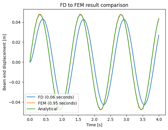
Here we will compare the two methods to each other and to a simplified analytical solution. The following conclusions can be drawn:
Even for a small number of elements (N = 10) the FD results are very closely related to the analystical solution.
The FEM results are a lot more accurate. However, they do take a lot longer to produce. The trade-off here is the ability to easier expand the FEM model to more complex shapes and boundary conditions.
The FEM results show some additional high-frequency peaks. This is a consequence of the relatively low number of elements.
t_FD = sol_FD.t
y_FD = sol_FD.y[int(len(sol_FD.y)/2)-1]
plt.plot(t_FD, y_FD, label=f"FD ({FD_EndTime-FD_StartTime:.2f} seconds)")

t_FEM = sol_FEM.t
y_FEM = sol_FEM.y[int(len(sol_FEM.y)/2)-1]
plt.plot(t_FEM, y_FEM, label=f"FEM ({FEM_EndTime-FEM_StartTime:.2f} seconds)")

# Simplified analytical -- assumption of static behaviour due to slow frequency
y_ana = P(t_FD)/E/A*L
plt.plot(t_FD, y_ana, label="Analytical")

plt.title("FD to FEM result comparison")
plt.legend(loc=3)
plt.xlabel("Time [s]")
plt.ylabel("Beam end displacement [m]");
Part 4: Other alternatives using other languages#
While Python is widely accepted as the future core of scientific programming, it is interesting to look at the options other programs provide as well. Within the academic community MAtlab and R are widely used. They benefit from years of development and accurate documantation, but lack some flexibility and are dissapearing from industry practices due to the lisence cost compared to upcoming alternatives. Additionally they are slower than python for most tasks. In view of programming alternatives to python are very broad. Due to their speed Fortran or C-based languages are widely used as well. They can be a factor 5 faster than python due to their compiler nature, but they are a lot less intuitive and thus harder to get into than python. As a solution the novel programming Language Julia tries to combine both these aspects. Below an example is added of the problem treated in this tutorial, only considered statically, but solved in Julia using the FEM package Gridap as well. Gridap internalized functions allow for the easy implementation of different shapes in FEM, at only a fraction of the computational cost. Similar to this one-end clamped rod, take a look at this complex geometry example of a 2-hole structure.